- Biomedical Research (2015) Volume 26, Issue 3
Classification of brain MRI images using support vector machine with various Kernels.
M. Madheswaran and D. Anto Sahaya Dhas*Department of ECE, Rajas Engineering College, Vadakkankulam, Tirunelveli 627116, India
- *Corresponding Author:
- M. Madheswaran
Centre for Research in Image and Signal Processing
Mahendra Engineering College
Mallasamudram 637503
India
E-mail: madheswaran.dr@gmail.com
Accepted date: April 29 2015
Abstract
An enhanced classification system for classification of brain tumor from MR images using association of kernels with support vector machine is developed and presented in this paper. Oriented Rician Noise Reduction Anisotropic Diffusion filter is used for image denoising. A modified fuzzy c-means algorithm termed as Penalized fuzzy c-means algorithm is used for image segmentation. The texture and Tamura features are extracted using GSDM and Tamura method. Genetic algorithm with Joint entropy is adopted for feature selection. The classification is done by support vector machine along with various kernels and the performance is validated. A classification accuracy of 98.83% is obtained using SVM with GRBF kernel.
Keywords
ORNRAD filter, Penalized Fuzzy C-means, genetic algorithm, SVM classifier, MRI images and Brain tumor.
Introduction
In recent years, brain tumor is found as one of the major diseases leading to death of human beings. The MRI is widely used by most of the physicians to identify the brain tumor in the present days. Identification of the tumor regions accurately from the MRI images is considered to be a challenging job for the physicians. The image processing tools are used to accurately classify the tumor. Many researchers reported various techniques for identification of tumor region.
Quantitative analysis on MRI brain image yields significant performance in noise reduction compared to other quality measures. Similarly, an anisotropic diffusion method for ultrasound images was explained using a novel filtering technique that relies on estimation of the standard deviation of the noise proposed by K.Krissian et al.,[1]. From the estimated noise, the metrics of the filter were chosen automatically. This property provided an intuitive filtering by enhancing the convergence rate of the diffusion. The parameters namely planar, volumetric and linear components of the image are combined in this filter.
Anand et al.,[2] proposed a bilateral filtering scheme based on wavelet in order to reduce the noises in MR images. The noisy coefficient utilized was undecimated Wavelet Transform (UWT). The efficiency of the denoising is enhanced by Bilateral filtering of the approximate coefficients. This method of denoising scheme was widely adapted to Rician noise. Moreover, the visualization and the diagnostic quality of the denoised image are enhanced by this filtering scheme. This scheme encompasses greater ability for noise suppression. Among the various denoising methodologies for MR images, tracking algorithm proposed by Jaya et al.,[3] for denoising the MR brain images. According to this algorithm, application of preprocessing technique provides more promising results. The algorithm processes the task in three stages namely, dataset acquisition, preprocessing and noise removal.
Yong Yang [4] proposed a novel fuzzy C-means algorithm named as Penalized fuzzy C-means algorithm. A penalty term is introduced by modifying the objective function of the general FCM. This approach overcomes the noise sensitiveness of the FCM. A high speed parallel fuzzy Cmeans algorithm was introduced by S.Murugavalli et al., [5]. It combines the advantages of both SFCM and PFCM. This algorithm reduces the execution time for large images.
Earlier methods used Spatial Gray Level Dependence Method (SGLDM) for feature extraction. Though it was successful, the time consumed by this method was higher and also has higher complexity. To reduce the time for computation A.E.Svalos et al., [6] analyzed the SGLDM method by a pilot application. A technique was proposed by M.Vasantha et al., [7] for extracting the intensity histogram and Gray Level Co-occurrence Matrix (GLCM) features from MR mammogram image.
Kernel F-force feature selection (KFFS) method was proposed by Kemal Polat et al., [8] for selecting the features. Results showed that the proposed KFFS functions better than the F-score feature selection. Followed by this, Hsieh-Wei Lee et al., [9] proposed a method for extracting the features from the brain images. This was carried out through integrating the Support Vector Machine (SVM) with the feature selection process in the kernel space. A new method was introduced by Bacauskiene.M et al., [10] in order to elect the salient features for classification and further image processing process. Here, paired t-test was used to eliminate the redundant features and a generic search was employed to detect the hyper-parameter, and to elect the salient features.
A texture based classification system was proposed by Sidhu et al.,[11] using SVM and wavelet transform. The core concept of this classification system was to identify and analyze the factors that considerably affect the performance of SVM and wavelet transform during the process of texture classification. A batch type learning vector quantization technique for segmentation was proposed by Miin-Shen Yang et al., [12]. It provides good accuracy and quality for the accurate measurement of hippocampus volume in MR images. The methodology was compared with the generalized Kohenen’s competitive learning method.
A hybrid technique based on association rule mining with decision tree algorithm was proposed by P.Rajendran et al., [13] for the classification of tumor from CT images. The image was segmented using morphological opening and edge detection techniques. Mubashir Ahmad et al., [14] reported a classification technique based on SVM classifier. The feature extraction was carried out by DAUB-4 wavelet and the features are selected using PCA. Linear kernel and Radial basis kernel functions of SVM were used for the classification. A performance analysis of the SVM classifier on brain tumor diagnosis was reported by P.Shantha Kumar et al., [15]. In this work the GLCM features, LBP features, Gray level features and Wavelet features are extracted and trained using SVM.
Amita Kumari et al., [16] proposed a hybrid method using PSO and SVM. Here the wavelet based texture features are extracted using HAAR wavelet. The features are then selected using PSO and trained with SVM. Anamika Ahirwar [17] provided information about the various segmentation and computation techniques which suits for the classification of brain MRI. Here the results were compared with the Keith’s database to show the prediction accuracies. Mehdi Jafari et al., [18] proposed a hybrid technique for automatic brain tumor detection. In this work the SVM classification technique was adopted for classification along with genetic algorithm.
Brain tumor classification using GA and SVM
The general flow diagram for the proposed work is shown in fig.1. The MR brain image under testing undergoes various processes such as preprocessing, feature extraction, feature selection and classification.

Figure 1: Flow graph of the brain tumor classification system
The preprocessing starts with the denoising of MR images.
It is accomplished by Oriented Rician Noise Reduction
Anisotropic Diffusion filter. It is a modified form of anisotropic diffusion filter which removes the rician noise
in MRI images without affecting the quality of the interesting
regions and preserves the edges. The MRI images
are denoted as random vector variables in which the unknown
random vector variables are denoted as x and the
known random vector variables are denoted as y. The estimation  of x is a function of y.
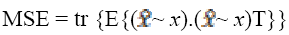
The estimated error vector (e) is equal to the difference of and x, while the MSE is equal to the trace of error covariance
matrix.
 (1)
(1)
where T is the structural tensor. A Linear MMSE (Minimum Mean Square Error) estimator is applied to minimize the MSE in the MRI images. An extension is applied to the matrix diffusion which possess the statistical properties of the local structure in the image which further improves the overall performance of the filter. Structure tensor can be described by the outer product of the gradient, smoothened by a Gaussian convolution as
 (2)
(2)Here  is a Gaussian kernel of standard deviation
  and
and  is the gradient of the output signal. Let,
ev1≥ ev2 ≥ ev3 ≥ 0 are eigenvalues and E1, E2, and E3 are
corresponding eigenvectors. The eigenvectors E1 and E3 provide the local orientation of maximal and minimal intensity
variation respectively.
is the gradient of the output signal. Let,
ev1≥ ev2 ≥ ev3 ≥ 0 are eigenvalues and E1, E2, and E3 are
corresponding eigenvectors. The eigenvectors E1 and E3 provide the local orientation of maximal and minimal intensity
variation respectively.
A diffusion matrix DM is designed to share eigenvectors 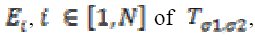 of , while the eigenvectors E1, E2
and E3 are related to leveling of noise. Then the eigenvectors
are written as
of , while the eigenvectors E1, E2
and E3 are related to leveling of noise. Then the eigenvectors
are written as
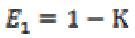 (3a)
(3a)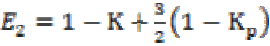 (3b)
(3b)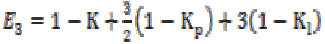 (3b)
(3b)where K is the gain coefficient in a local isotropic
neighborhood,  is the
gain in the local planar neighborhood defined by the eigenvectors
E2 and E3, and
is the
gain in the local planar neighborhood defined by the eigenvectors
E2 and E3, and 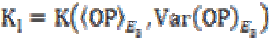 is the gain in the local linear neighborhood oriented by
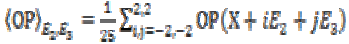
eigenvector E3. Then the local mean value can be calculated
as
is the gain in the local linear neighborhood oriented by
eigenvector E3. Then the local mean value can be calculated
as
 (4)
(4)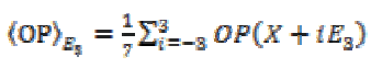 (5)
(5)Here same sets of neighborhood, are used to compute the local variance. The diffusion matrix (DM) can be written upon the basis of (E1, E2, E3) as
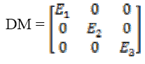 (6)
(6)Equation (7) shows the corresponding diffusion equation as a sum of three diffusion terms.
 (7)
(7) is the projection of the gradient formed by
  and
and  is the projection of the gradient
in the direction E3. A multithreaded version of
Jacobi numerical scheme is used for the discretization
of Partial Differential Equation.
is the projection of the gradient
in the direction E3. A multithreaded version of
Jacobi numerical scheme is used for the discretization
of Partial Differential Equation.
(8)Here ž is the neighborhood of the point X. is the mean
value of diffusion coefficient between the position X and
its neighbor pixel n. It is stable for any time step
is the mean
value of diffusion coefficient between the position X and
its neighbor pixel n. It is stable for any time step  and
also has better convergence time. The primary reason for
choosing the ORNRAD filter is due to the minimum filtering
time compared with other filters. This filter results in an efficient reduction of noise simultaneously preserving
the detailed components and the high definition of the
interface between various brain tissues.
and
also has better convergence time. The primary reason for
choosing the ORNRAD filter is due to the minimum filtering
time compared with other filters. This filter results in an efficient reduction of noise simultaneously preserving
the detailed components and the high definition of the
interface between various brain tissues.
Segmentation is an important process in MRI image classification in which the testing area is extracted from the whole image. Here it is done by adopting an algorithm termed as Penalized Fuzzy C-Means algorithm (PFCM) which is a modified FCM algorithm. In conventional FCM algorithm, there is no information about spatial context, which cause it to be sensitive to noise and imaging artifacts. In PFCM, a penalty term considers the spatial dependence of the object which is inspired by the Neighborhood Exception maximization algorithm and is modified according to the FCM criterion. The objective function of the PFCM is given by
(9)where (10)  Controls the effect of the penalty term.
The objective function  can be minimized with the
help of an iterative algorithm which is derived by the
valuation of the centroids and membership functions that
satisfy a zero gradient condition. When the PFCM algorithm
converges, a defuzzification process takes place to
convert the fuzzy partition matrix into a crisp partition
which is the segmented image.
can be minimized with the
help of an iterative algorithm which is derived by the
valuation of the centroids and membership functions that
satisfy a zero gradient condition. When the PFCM algorithm
converges, a defuzzification process takes place to
convert the fuzzy partition matrix into a crisp partition
which is the segmented image.
Visual content in the image are captured by extracting the features present in the image. This information is useful for the indexing and retrieval. Visual features are lowlevel or primitive features, which can be either domainspecific such as human face, finger prints, etc. or general features like color, shape, and texture. Features can be extracted based on color, texture, or shape. The texture based features are extracted in the present work. The texture can be characterized by structure (spatial relationship) and tone (intensity property). This is implemented through the GSDM and Tamura method. Tamura features of a preprocessed image can be retrieved through constructing a co-occurrence matrix named Gray Level Cooccurrence Matrix (GLCM) also known as GSDM.
This matrix is a two dimensional matrix Pd, which holds the information about the position of the pixel that has similar brightness value (gray levels). Pd considers and specifies the relationship among the reference and neighbour pixel at a time. Neighbour pixels, which are presented at the right side of the reference pixel, which is expressed using P(i, j) relation. It has n x n dimension, where n denotes the number of gray levels in the image. Number of occurrence of the image can be represented in the matrix as nij. Likewise, value (i, j) is lying at distance d in the image. For example, if d = (1, 1) then they are found from the matrix as shown in Fig. 2.

Figure 2: Co-occurrence matrix

Figure 3: Noisy input image and denoised output image of ORNRAD filter
It contains 16 pairs of pixels that satisfies the separation in spatial. In the example as there are only 3 gray levels the P(i, j) is of 3 x 3 matrix. Following steps are carried out to construct the co-occurrence matrix
1. Pairs of pixel are counted, in which the value of i (i.e. the first pixel) and j (i.e. i’s matching pixel) are situated at a distance d.
2. The computed count is inserted into the matrix at ith row and jth column Matrix is not symmetric, due to the number of pixel pairs having gray level is not necessarily equal to the number of pairs of pixel having gray level.
Different texture and Tamura features can be extracted to predict the risk level of the tumor. Each feature value can be computed from the matrix constructed using their corresponding formulas and they are used to analyze different properties of an image separately. These features, explain the spatial ordering of texture constituents.
(i) Contrast
Local variance present in the brain tumor MRI can be measured using contrast. If P (i, j) in the matrix has more variations then the contrast will be high. The contrast value from the matrix can be obtained from
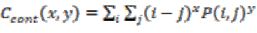 (11)
(11)(ii) Homogenity
The homogeneity of an image can be found from the combination of low and high values of P(i, j) in the cooccurrence matrix. This feature results in spreading the P(i, j) values evenly in the matrix. Mathematically homogeneity can be expressed as
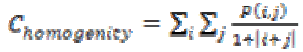 (12)
(12)(iii) Entropy
This is a measure of information content and randomness of intensity distribution. When all the entries of the matrix are of same magnitude then entropy is higher otherwise, it is smaller. The entropy can be measured using the equation (13).
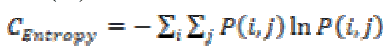 (13)
(13)(iv) Correlation
Intensity of an image is measured using Correlation through the equation (14). If an image contains a considerable amount of linear structure then the correlation value will be higher.
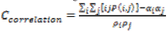 (14)
(14)Where, 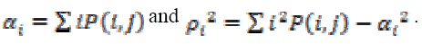
(v) Energy
The Texture energy is measured by
 (15)
(15)(vi) Maximum Probability
This feature corresponds to the strongest response. This can be expressed mathematically as
 (16)
(16)(vii) Local Homogeneity, Inverse Difference Moment (IDM)
This is influenced by the feature homogeneity of an image. IDM values are low for the inhomogeneous images and high for homogeneous images. It can be measured as
 (17)
(17)(viii) Sum of square, variance
The element whose values differ greatly from the P(i,j)’s average value then for such elements the feature values are relatively high value. It can be computed as
 (18)
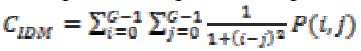
(18)(ix) Auto correlation
Coarseness and regularity of an images texture can be analyzed through Kaizer. Spatial relationship among the primitives can be measured using
 (19)
(19)(x) Directionality
Total degree of directionality is calculated for the neighbours that are non-overlapping using
 (20)
(20)(xi) Coarseness
This feature is calculated for each pixel (x, y) in the image using the equation (21). This represents the direct relationship to the repetition rate and scale.
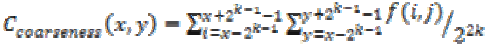 (21)
(21)Other features
1. Cluster Shade:
 (22)
(22)Where, 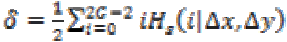
2. Cluster Prominence:
 (23)
(23)3. Inertia :
 (24)
(24)4. Cluster tendency:
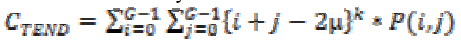 (25)
(25)The subset of features can be selected for dimensionality reduction from the extracted features. This is normally carried out in order to eliminate redundant and irrelevant features that are extracted. The selection process is carried out using joint entropy and genetic algorithm. The entropy is estimated for the features and for the target of the selected image that required to be predicted. This value is determined from a grayscale image, which measures the randomness present in the image to characterize the input image’s texture. Having entropy values determined the mutual information among the features and targets are determined. This information is used to estimate and measure how a random variable is able to describe and impact on other variable.
With this statistical information, genetic algorithm is implemented to estimate the fitness values for all the extracted features from the population initialization. The determined fitness values are analyzed to determine whether the minimum relevance and maximum redundancy exits between the features that are extracted. If it fails to choose a feature subset then they are processed again by the genetic algorithm. Otherwise, the chosen features are grouped to form a subset based on which prediction process is carried out.
Classification is the process of classifying the given input by training with a suitable classifier. Support Vector Machine (SVM) classifier is one of the best classifier suggested by many researchers which can be opted for the brain tumor classification from MR images. It is independent of dimensionality and feature space. SVM transforms the input space to a higher dimension feature space through a non-linear mapping function and construct the separating hyperplane with maximum distance from the closest points of the training set. SVM classifier along with linear and non-linear kernel functions produces best results in classification. It is found that the seven kernels mentioned here can be used for MR image classification.
1. Linear kernel:
The linear kernel is the simplest kernel. It is defined by
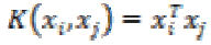 (26)
(26)2. Polynomial kernel:
The polynomial kernel is suited for problems with normalized training data.
It is given by (27)
(27)
where α is the slope, c is a constant and d is the polynomial degree.
3. Gaussian Radial Based Function kernel:
The GRBF kernel is defined as
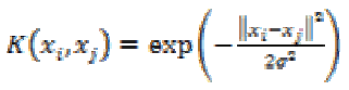 (28)
(28)where σ is an adjustable parameter. It is a non-linear kernel and is very sensitive to noise.
4. Exponential Radial Based Function kernel:
The ERBF kernel is close to GRBF with only the square of the norm removed. It is defined as
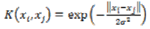 (29)
(29)5. ANOVA kernel:
The ANOVA kernel is also a radial based function kernel. It is defined as
 (30)
(30)6. Multilayer Perceptron kernel:
Multilayer Perceptron kernel is also called as Hyperbolic Tangent kernel or Sigmoid kernel. It is defined as
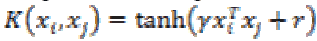 (31)
(31)where γ is the slope and r is the intercept constant.
7. Fisher kernel: Fisher kernel is defined is
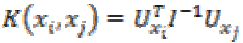 (32)
(32)Results and Discussion
The classification of MRI brain images using PFCM, GA and SVM with kernels is carried out using image processing tools. The images are taken from the databases namely MR-TIP, NCIGT, BraTS, BITE and TCIA. The images are preprocessed for noise removal, segmented for separation of interesting area and the features are extracted for classification. The performance of the ORNARD filter is estimated and compared with various filters as shown in Table 1 and is further used for validation. The denoised image is then segmented for extracting the area of interest from the image. The skull region and other unwanted regions were removed using Penalized Fuzzy C-means algorithm. The segmentation accuracy of PFCM algorithm for 10 images is compared with other Fuzzy based segmentation algorithms and the result is given in Table 2. The PFCM algorithm performs well by consuming a minimal time compared to other fuzzy algorithms. Then the segmented image is subjected to feature extraction. The extracted texture and Tamura features are then subjected to feature selection which is done by Genetic algorithm along with Joint entropy. The extracted feature values for a sample image are given in Table 3.

Table 1: Performance comparison of various filters

Table 2: Performance comparison of various Fuzzy based segmentations

Table 3: Extracted values for the features
The output of the GA is then trained with SVM classifier using seven types of kernels. The polynomial kernel is also tested with the degree from 1 to 5. For the GRBF, ERBF and ANOVA kernels it is tested with the scaling factor from 1 to 5. Here the performance of the present method was evaluated in terms of sensitivity, specificity and accuracy.
Sensitivity is the probability of positive for a diagnostic test. It is also termed as true positive fraction. The percentage of sensitivity is given by

where is the True positive and
 is the False negative.
Specificity is the probability of negative for a diagnostic
test. It is also termed as true negative fraction. The percentage
of specificity is given by
is the False negative.
Specificity is the probability of negative for a diagnostic
test. It is also termed as true negative fraction. The percentage
of specificity is given by
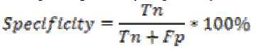
where is the True negative and
  is the False positive.
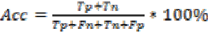
Accuracy is the probability that a diagnostic test is correctly
performed. It is calculated by
is the False positive.
Accuracy is the probability that a diagnostic test is correctly
performed. It is calculated by
The performance of the SVM classifier with various kernels is given in Table 4. From the table it is found that the SVM classifier with GRBF kernel performs better than the other kernels. It is also estimated 100% sensitivity, 90% specificity and accuracy of 98.83% for the SVM classifier with GRBF kernel. This may be due to the inherent property of gradient in GRBF kernel.

Table 4: Performance of various kernels with SVM
The classifications of the MR image using various kernels are given in Table 5. It is found that the GRBF kernel classifies the tumor more accurately than the other kernels.

Table 5: Classification of MR image based on the kernels
The performance of the developed classification system is compared with the existing techniques is given in the Table 6.

Table 6: Comparison of Classification Accuracy Obtained by Various Methods
It is seen that the SVM classifiers outperform other classifiers. In particular, the SVM classifier with GRBF kernel produces a higher classification accuracy of 98.83%. This is due to the combination of the ORNRAD filter smoothing characteristics and GRBF kernel for classification.
Conclusion
An efficient brain MR images classification technique using support vector machine with kernels is proposed in this paper. The features are extracted using Penalized fuzzy C-means algorithm and the optimized features are selected using genetic algorithm along with joint entropy. The performance of SVM classifiers with various kernels was estimated and found that the GRBF kernel performs well compared to other kernels. The classification accuracy was also found to be high for SVM classifier with GRBF kernel.
References
- Krissian K, Aja-Fernández S. Noise-driven anisotropic diffusion filtering of MRI. Image Processing, IEEE Transactions on 2009; 18: 2265-2274.
- Anand CS, Sahambi JS. Wavelet domain non-linear filtering for MRI denoising. Magnetic Resonance Imaging 2010; 28: 842-861.
- Jaya J, Thanushkodi K, Karnan M. Tracking algorithm for de-noising of MR brain images. International Journal of Computer Science and Network Securit 2009; 9: 262-267.
- Yong Yang. Image segmentation by Fuzzy C-means clustering algorithm with a novel penalty term. Computing and Informatics 2007; 26: 17-31.
- S Murugavalli, V Rajamani. A high speed parallel fuzzy C mean algorithm for brain tumor segmentation. BIME journal 2006; 6(1).
- Svolos A E, Todd-Pokropek A. Time and space results of dynamic texture feature extraction in MR and CT image analysis. IEEE transactions on journal of information technology in Biomedicine 1998; 2(2): 48-54.
- Vasantha M, Subbiah Bharathi V, Dhamodharan R. Medical Image Feature, Extraction, Selection and Classification. International Journal of Engineering Science and Technology 2010; 2(6): 2071-2076.
- Kemal Polat, Salih Gunes. A new feature selection method on classification of medical datasets: Kernel Fscore feature selection. International Journal of Expert Systems with Applications 2009; 36(7): 10367-10373.
- Hsieh-Wei Lee, King-Chu Hung, Bin-Da Liu, Sheau- Fang Lei, Hsin-Wen Ting. Realization of High Octave Decomposition for Breast Cancer Feature Extraction on Ultrasound Images. IEEE transactions on Circuits and System 2011; 58(6): 1287-1299.
- Bacauskiene M, Verikas A, Gelzinis A, Valincius D. A feature selection technique for generation of classification committees and its application to categorization of laryngeal images. Journal of Pattern Recognition 2009; 42(5): 645-654.
- S Sidhu, K Raahemifar. Texture classification using wavelet transform and support vector machines. Electrical and Computer Engineering Canadian Conference proceeding 2005; 941-944.
- Miin-Shen Yong, Karen Chia-Ren Lin, Hsiu-Chih Liu, Jiing-Feng Lirng. Magnetic resonance imaging segmentation techniques using batch type learning vector quantization algorithms. Magnetic Resonance Imaging 2007; 25: 265-277.
- P Rajendran, M Madheswaran. Hybrid medical image classification using association rule mining with decision tree algorithm. Journal of Computing 2010; 2(1).
- Mubashir Ahmad, Mahmood ul-Hasan, Imran Shafi, Abdelrahman Osman. Classification of tumors in human brain MRI using wavelet and support vector machine. IOSR Journal of Computer Engineering 2012; 8(2): 25-31.
- P Shantha Kumar, P Ganesh Kumar. Performance analysis of brain tumor diagnosis based on soft computing techniques. American Journal of Applied Sciences 2014; 11(2): 329-336.
- Amita Kumari, Rajesh Mehra. Hybridized classification of brain MRI using PSO and SVM. International Journal of Advanced Technology 2014; 3(4).
- Anamika Ahirwar. Study of techniques used for medical image segmentation and computation of statistical test for region classification of brain MRI. I.J.Information Technology and Computer Science 2013; 5: 44-53.
- Mehdi Jafari, Reza Shafaghi. A hybrid approach for automatic tumor detection of brain MRI using support vector machine and genetic algorithm. Global Journal of Science, Engineering and Technology 2012; 3: 18.
- E A El-Dihshan, T Hosney, A B M Salem. Hybrid intelligence techniques for MRI brain image classification. ELSEVIER, Digital Signal Processing 2010; 20: 433-441.
- Ahlam Fadhil Mahmood , Ameen Mohammed Abd- Alsalam. Automatic brain MRI slices classification using hybrid technique. Al-Rafidain Engineering 2014; 22(3).
- N Rajalakshmi, V Lakshmi Prabha. Automated classification of brain MRI using color converted K-means clustering segmentation and application of different kernel functions with multi-class SVM. Proceedings of 1st annual international interdisciplinary conference