Review Article - Journal of Psychology and Cognition (2017) Volume 2, Issue 2

Mathematics of the brain: generalization from Eigen vectors to eigen functions.

Thomas Saaty^*

Center of the Philosophy of Science, University of Pittsburgh, USA

*Corresponding Author:

Thomas Saaty
Distinguished University
Professor Fellow of the Center of the Philosophy of Science
University of Pittsburgh, USA
Tel: 0014126216546
E-mail: saaty@katz.pitt.edu

Accepted date: June 05, 2017

Citation: Saaty T. Mathematics of the brain: generalization from Eigen vectors to eigen functions. J Psychol Cognition. 2017;2(2):113-122.

Abstract

In this paper, we provide an overview of the mathematics of the brain and present the generalization from Eigen vectors to Eigen functions. Initially we summarize some of the mathematics of derived priority scales involved in the multicriteria decision process, and give the corresponding generalization to the continuous case. Then we discuss of density and approximation and how we can generalize from discrete to continuous judgments. The solutions of the functional equation w(as)=bw(s) are given in the real and complex domain and then for quaternions (non-commutative) and octonions (non-commutative and non-associative). In the end we present the consequences and evidence for validation: a) The Laws of Nature are written in the Workings of our Brains, b) the Weber-Fechner Law of Psychophysics, and c) The Brain Works with Impulsive Firings.

Keywords

Nervous system, Brain, Mathematics.

Introduction

It is useful to summarize some of the mathematics of derived priority scales involved in the multicriteria decision process, and give the corresponding generalization to the continuous case. First we examine the solvability of a system of linear algebraic equations given in matrix form. The homogeneous system Ax = 0 has a non-zero solution if A has no inverse A⁻¹ with AA⁻¹ = A⁻¹A = I , where A is the identity matrix and hence the determinant of A is equal to zero. The inhomogeneous system Ax = y has a solution x = A⁻¹y if A⁻¹ exists. This means that the determinant of A is not zero. We recall that an Eigen value λ of A is a root of the characteristic equation of A and that a right Eigen vector of A is a solution x of the equation Ax = λ x. This can also be written as (λ I − A)x = 0. A homogeneous Eigen value system (λ I − A)x = 0 has a solution if the determinant of (λ I − A) which is a polynomial (the characteristic polynomial) in λ is equal to zero which is true only if λ is a zero of that polynomial. That value of λ is an Eigen value of the matrix A. The inhomogeneous system (λ I − A)x = y has a solution x = (λ I − A)−1 y if (λ I − A)⁻¹exists which it does only when λ is not an Eigen value of A. The set of Eigen values of A is the spectrum of A. It is clear that A is the kernel or focus that provides the conditions for the system of equations to have or not have a solution. These ideas will be relevant in the ensuing generalization to the infinite case.

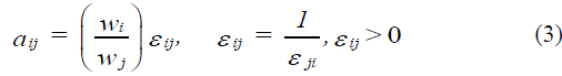
Our approach uses absolute numbers, invariant under the identity transformation. We must filter or interpret the intensities of magnitudes of numbers in terms of our own sense of importance. We can use absolute numbers to construct a fundamental scale of priorities across all dimensions of experience by making paired comparisons of two elements at a time using the smaller one as the unit and estimating the larger one as a multiple of that unit with respect to a common property or criterion that they have in common. From such paired comparison, we can then derive an overall priority scale of relative importance for all the elements. Finally, we combine such priority scales with respect to different criteria by weighting each by the weight of the corresponding criterion and adding over the criteria to obtain a priority scale of measurement for all the elements with respect to all the criteria. One cannot escape the fact that one can only add and multiply such priority scale numbers, but not with numbers that belong to ordinal or interval scales nor to ratio scales that need a standard unit for measuring all priorities. The expression we encountered for deriving an absolute scale to make pairwise comparisons applies to the case of making a finite number of judgments is:

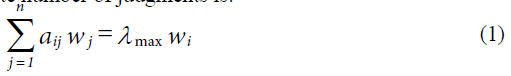
with a_ji=1/a_ij or a_ij a_ji=1 (the reciprocal property), a_ij>0 (thus A is known as a positive matrix) whose solution is normalized so that,

When 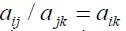the matrix is consistent and its maximum Eigen value is equal to n. Otherwise, it is simply reciprocal. A is consistent if and only if 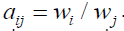This is the central ratio scale property of a consistent matrix. What is powerful about a ratio scale when dealing with tangibles is that in normalized form it has the same value no matter what is its original multiplier. Thus two batches of bananas that weigh 3 and 6 kg, on normalization, have the relative weights 3/(3+6)=1/3 and 6/(3+6)=2/3. These two batches also have the weight in pounds of 6.63 and 13.26, respectively. When normalized, these weights are again 6.63/(6.63+13.26)=1/3 and 13.26/(6.63+13.26)=2/3. Thus, when normalized, ratio scales reduce to a standard form. In addition, the ratio of two numbers taken from the same ratio scale is an absolute number.

If A is simply reciprocal and positive, but not consistent that is 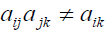does not hold for some i, j and k and we must have:

A left Eigen vector y of A is a solution of the equation yA = λ y. For a consistent matrix, the corresponding entries of the normalized left and right Eigen vectors are reciprocals. The reason why we used the principal right Eigen vector only in the discrete case, is because in making paired comparison judgments one must identify the smaller or lesser element and use it as a unit and then estimate how many times of that unit the larger element dominates it in value. We cannot tell what fraction of the larger element the smaller one is without first using it as the unit. Knowing that the left and right Eigen vectors are reciprocals when we have consistency will be useful in the continuous case where if we wish we could construct two matrices corresponding to each of the left and right Eigen functions approaches.

We note that the reciprocal axiom of paired comparisons involves division. Because making comparisons is:

1) The most fundamental principle in relating entities for better understanding,

2)The brain works with electric signals that need complex numbers for explanation and understanding. These signals can be measured and compared again using reciprocal comparisons, and

3) Also perhaps the brain works at its synapses with signals whose chemical nature is not yet fully understood that again can be compared according to their relative intensities and involve paired reciprocal comparisons. It is necessary for conscious understanding of phenomena according to the accurate workings of the brain in making comparisons that division should always be possible. This leads us to a brief discussion of division algebras and hyper-complex numbers.

In 1898 Adolf Hurwitz proved there are exactly four normed division algebras: the real numbers (R), the complex numbers (C), the quaternions (H) and the octonions (O).

Immediately beyond those four are the sedenions and beyond (in fact, one can get an algebra of 2n for any nonnegative n), but these algebras are perhaps less interesting because they are no longer division algebras—that is, ab = 0 no longer implies that either a = 0 or b = 0. Quaternions, discovered by the Irish mathematician William Rowan Hamilton in 1843 are an alternative method of handling rotations, besides rotation matrices. The advantage of quaternions over other representations is that they allow interpolation between two rotations. Another way to say what special about 2 dimensions are is that rotation commutes, but not in 3 or more dimensions. Thus, there is advantage to the fact that quaternions do not commute. Inspired by Hamilton, John T Graves, from Britain discovered in 1843 what he called the octaves (later called octonions) and communicated by mail to Hamilton who promised him to take it up before the Academy in Dublin, but forgot to do it immediately. They were discovered independently and published first in 1845 by Arthur Cayley. Octonions were sometimes referred to as Cayley numbers or the Cayley algebra.

With quaternions we lose the commutative law, with octonions we also lose the associative law. It was the prodigious Hamilton who first noticed that multiplication of octonions is not associative, that is, a ×(b × c) does not equal to (a ×b) × c. The main thing we are left with is the ability to divide in order to give meaning to proportionality. The solutions to our operator equation do not extend to quaternions and octonions when the parameters and the variables belong to these algebras. An exception is when they are real or complex.

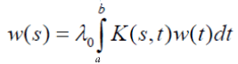
Let us generalize further the mathematics of the fundamental idea of an infinite number, a continuum, of pairwise comparisons [1]. This leads us from the solution of a finite system of homogeneous equations or alternatively, and according to the theory of Perron, to raising a positive reciprocal pairwise comparisons matrix to limiting powers to obtain its principal Eigen vector, to the solution of a Fredholm equation of the second kind to obtain its principal Eigen function. A necessary condition for the existence of this Eigen function w(s) is that it is the solution of the functional equation w(as) = bw(s) Surprising and useful properties of this solution emerge and are related to how our brains respond to stimuli through the electrical firing of neurons and how bodies in the universe responding to each other’s influence satisfy a near inverse square law discovered in physics - the principle that responding to influences in a manner that satisfies a natural law is an attribute of all things be they material or mental. We believe that it is the kind of understanding that drove the very insightful Julian Huxley [Man in the modern world (1947)] to write that “something like the human mind might exist even in lifeless matter.” It is the vital force called Qi that in Taoism and other Chinese thought is thought to be inherent in all things. The unimpeded circulation of Qi and a balance of its negative and positive forms in the body are held to be essential to good health in traditional Chinese medicine. Thus all things that exist respond to stimuli to a larger or smaller extent as our mind does.

The idea to generalize the formulation of the judgment process to the continuous case, to Fredholm’s equation of the second kind is carried out in two ways. The first is by starting from the beginning to develop the equation. The second is by generalizing the discrete to the continuous formulation. Both yield the same answer. It turns out that the functional equation w(as) = bw(s) (which we developed several years prior to this analysis through the intuitive observation about the proportionality of response to stimuli w(as) ∝ w(s) ) as a necessary condition for the existence of a solution to Fredholm’s equation. I worked with one of the world’s leading mathematician in functional equations, Janos Aczel of the University of Waterloo, with whom I had published a paper showing that the geometric mean is necessary for combining individual reciprocal judgments into a representative group judgment [2]. This result I had already known and used in my works without a comprehensive proof. Aczel was both my helper and tutor in pressing forward in my work using this rather simple but powerful functional equation to continue the generalization of the process of decision making to the continuous case. Finally, my generalization of the linear equation w(as) = bw(s) to an equation in operators involving functions rather than variables, whose solution was once said to be very difficult to obtain, was actually solved by Nicole Brillouet-Belluot of the École Centrale de Nantes, France [3]. Her solution has useful implications for relating our judgment mechanism to all works in science because it directs us to define the world as we sense and experience it to the response organs we have in our nervous system and imagination to grasp its meaning.

Density and Approximation

The utility of artificial neural network models lies in the fact that we use them to infer a function from observations. The brain itself has its system to determine the functions it needs to capture its perceptions and thoughts.

Approximation theory is concerned with approximating functions by simpler and more easily calculated functions. The first question we ask in approximation theory concerns the possibility of approximation. Is the given family of functions that we use for approximation dense in the set of functions to be approximated? Although continuous functions contain many pathological examples and deficiencies, every such function can be approximated arbitrarily close by polynomials, considered the best kind of smooth function. Approximation is about how general functions can be decomposed into more simple building blocks: polynomials, splines, wavelets, and the like. One needs to guarantee specified rates of convergence when the smoothness of the kind of functions being approximated is specified, such as in Sobolev or Lipschitz spaces. A function f (x) belongs to a Lipschitz class Lip[α] if there exists a constant C>0 such that |f (x) – f (y)| ≤ C |x-y|α.

The General Problem of Approximation: Let x be a metric space and k a subset of x. For a given point xε X define d (x,k)=inf d (x,y) for y in k. The general problem of approximation is to find whether such a y exists for which the infimum is attained, and to determine whether it is unique or not. An element y₀ ε k for which the infimum is attained is called an element of best approximation to the element xε X (or simply, a best approximation). An alternative way of defining the problem is as follows: Let X is a normed linear space and Y a subspace of X. Given an element xε X, we wish to determine d (x,y)=inf ||x-y|| for y in Y and study the existence and uniqueness of the element(s) y₀, for which ||x-y₀||=d (x,y). The Fundamental Theorem of Approximation Theory (5) states that if Y is a finite dimensional subspace of a normed linear space X, then there always exists an element y₀ εY of best approximation for each x ε X. However, the element of best approximation may not be unique. Uniqueness can only be guaranteed if X is a strictly normalized space, i.e.:

The Weierstrass approximation theorem proved by Karl Weierstrass in 1885 says that a continuous function on a closed interval can be uniformly approximated as closely as desired by a polynomial function. The degree of the polynomial depends on the function being approximated and on the closeness of the approximation desired. Because polynomials are the simplest functions and computers can directly evaluate polynomials, this theorem has both practical and theoretical relevance. Weierstrass also proved that trigonometric polynomials are also be used to approximate to a continuous function that has the same value at both end point of a closed interval. That is trigonometric polynomials are dense in this class of continuous functions. Each polynomial function is approximated uniformly by another polynomial with rational coefficients. There are only countably many polynomials with rational coefficients.

For complex analysis, Mergelyan proved in 1951 that: If K is a compact subset of the complex plane C such that C\K (the complement of K in C) is connected, then every continuous function f: K→ C whose restriction to the interior of K is holomorphic, can be approximated uniformly on K with polynomials. It has been noted that Mergelyan's theorem is the ultimate development and generalization of Weierstrass theorem and Runge's approximation theorem in complex analysis which says that: If K is a compact subset of C (the set of complex numbers), A is a set containing at least one complex number from every bounded connected component of C\K, and f is a holomorphic function on K, then there exists a sequence (r_n) of rational functions with poles in A such that the sequence (r_n) approaches the function f uniformly on K. It gives the complete solution of the classical problem of approximation by polynomials.

In the case that C\K is not connected, in the initial approximation problem the polynomials have to be replaced by rational functions. An important step of the solution of this further rational approximation problem was also suggested by Mergelyan in 1952.

Marshall H Stone considerably generalized the theorem and later simplified the proof; his result is known as the Stone-Weierstrass theorem. Let K be a compact Hausdorff space and A is a sub algebra of C(K,R) which contains a non-zero constant function. Then A is dense in C(K,R) if, and only if, it separates points.

This implies Weierstrass' original statement since the polynomials on [a,b] form sub algebra of C[a,b] which separates points.

But the problem of approximation is even simpler in conception. David Hilbert noticed that all basic algebraic operations are functions of one or two variables. So, he formulated the hypothesis that not only one cannot express the solution of higher order algebraic equations in terms of basic algebraic operations, but no matter what functions of one or two variables we add to these operations, we still would not be able to express the general solution. Hilbert included this hypothesis as the 13th of his list of 23 major problems that he formulated in 1900 as a challenge for the 20th century.

This problem remained a challenge until 1957, when Kolmogorov proved that an arbitrary continuous function on an n-dimensional cube (of arbitrary dimension n) can be represented as a composition of addition of some functions of one variable. Kolmogorov’s theorem shows that any continuous function of n dimensions can be completely characterized by a one-dimensional continuous function. This is particularly useful in interpreting how the brain, which consists of separate neurons, can deal with multiple dimensions by synthesizing information acquired through individual neurons that process single dimensions. Kolmogorov's powerful theorem does not guarantee any approximation accuracy and his functions are very non-smooth and difficult to construct. In 1987, Hecht-Nielsen noticed that Kolmogorov’s theorem actually shows that an arbitrary function f can be implemented by a 3-layer neural network with appropriate activation functions. The more accurately we implement these functions, the better approximation to f we get. Kolmogorov's proof can be transformed into a fast iterative algorithm that converges to the description of a network, but it does not guarantee the approximation accuracy by telling us after what iteration we get it.

The existence of a neural network that approximates any given function with a given precision was proven by Hornik, Stinchcombe and White. The utility of artificial neural network models lies in the fact that they can be used to infer a function from observations. This is particularly useful in applications where the complexity of the data or task makes the design of such a function by hand impractical. Neural nets have been successfully used to solve many complex and diverse tasks, ranging from autonomously flying aircrafts to detecting credit card fraud.

In the artificial intelligence field, artificial neural networks have been applied successfully to speech recognition, image analysis and adaptive control, in order to construct software agents (in computer and video games) or autonomous robots. Most of the currently employed artificial neural networks for artificial intelligence are based on statistical estimation, optimization and control theory.

Neural networks, as used in artificial intelligence, have traditionally been viewed as simplified static models of neural processing in the brain, even though the relation between this model and brain biological architecture is very much debated. To answer this question, Marr has proposed various levels of analysis which provide us with a plausible answer for the role of neural networks in the understanding of human cognitive functioning.

The question of what is the degree of complexity and the properties that individual neural elements should have in order to reproduce.

Neural networks are made of units that are often assumed to be simple in the sense that their state can be described by single numbers, their "activation" values. Each unit generates an output signal based on its activation. Units are connected to each other very specifically, each connection having an individual "weight" (again described by a single number). Each unit sends its output value to all other units to which they have an outgoing connection. Through these connections, the output of one unit can influence the activations of other units. The unit receiving the connections calculates its activation by taking a weighted sum of the input signals (i.e., it multiplies each input signal with the weight that corresponds to that connection and adds these products). The output is determined by the activation function based on this activation (e.g. the unit generates output or "fires" if the activation is above a threshold value). Networks learn by changing the weights of the connections.

In modern software implementations of artificial neural networks the approach inspired by biology has more or less been abandoned for a more practical approach based on statistics and signal processing. In some of these systems, neural networks, or parts of neural networks (such as artificial neurons) are used as components in larger systems.

Generalizing from Discrete to Continuous Judgments

Although we believe that the continuous version described below came first through our biological evolution, the way we learn things in general goes from the simple to the more complex in order that our analytical minds can lay things out according to increasing order of complexity. To survive in the real world we have to make comparisons among a myriad of entities. It is easier for us to deal with the solution of the comparisons problem by going from the simpler to the more complex.

In this generalization it turns out that the functional equation w(as) = bw(s) is a necessary condition for Fredholm’s integral equation of the second kind to have a solution. Instead of a pairwise comparisons matrix one uses the kernel of an operator. Operations on the matrix translate to operations on the kernel. From the matrix formulation leading to the solution of a principal Eigen value problem:

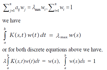
where the positive matrix A is replaced by a positive kernel K(s,t) > 0, a ≤ s,t ≤ b and the Eigen vector w by the Eigen function w(s). Note that the entries in a matrix depend on the two variables i and j that assume discrete values. Thus the matrix itself depends on these discrete variables and its generalization, the kernel function, depends on two (continuous) variables s and t. The reason for calling it a kernel is the role it plays in the integral, where without knowing it we cannot determine the exact form of the solution. The standard way in which the first equation is written is to move the Eigen value to the left hand side which gives it the reciprocal form. In general, by abuse of notation, one continues to use the symbol λ to represent the reciprocal value and with it one includes the familiar condition of normalization,

Here also, the kernel K (s,t) is said to be 1) consistent and therefore also reciprocal, if K (s,t) K (t,u)=K (s,u), for all s, t and u, or 2) reciprocal, but perhaps not consistent, if K(s,t)K(t, s) =1 for all s,t.

A value of λ for which Fredholm’s equation has a nonzero solution w (t) is called a characteristic value (or its reciprocal is called an Eigen value) and the corresponding solution is called an Eigen function. An Eigen function is determined to within a multiplicative constant. If w (t) is an Eigen function corresponding to the characteristic value λ and if C is an arbitrary constant, we see by substituting in the equation that Cw (t) is also an Eigen function corresponding to the same λ. The value =0 is not a characteristic value because we have the corresponding solution w (t)=0 for every value of t, which is the trivial case, excluded in our discussion.

Thus, we select an interval of time [a,b] and our convention will be to choose a=0. Let be a partition of the interval Let w be a single firing (voltage discharge) of neuron in spontaneous activity. In simple terms, if G(t),t∈[0,b] is the cumulative response of the neuron in spontaneous activity over time, given by 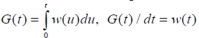where w(t) dt is the response during an infinitesimal period of time. Note that G (t) is monotone increasing and hence w (t)>0 and w(0)=0. Let

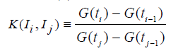
be the relative comparison of the response of a neuron during a time interval of length . with another time interval of length Cross multiplication and summation over j yields

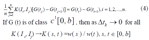
Also because the left-hand side of (1) is an average, we obtain as for all k, and as

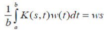
It is easy to show that b is the principal Eigen value (i.e., the largest in absolute value) of the consistent kernel K (s, t) because all the other Eigen values are zero (the Eigen functions being any function orthogonal to w (t) on [0, b] In general, if is reciprocal but not consistent, the homogeneous equation takes the form

or in operator form

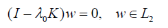
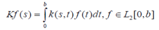
where I is the identity operator and K is a compact integral operator defined on the space of Lebesgue square integrable functions:

Because positive reciprocal kernels are non-factorable (the property that corresponds to irreducibility for nonnegative matrices), there exists a unique positive simple Eigen valuewhose modulus dominates the moduli of all other Eigen values.

As in the discrete case, there is an Eigen function w (s) that is unique to within a multiplicative constant, which corresponds to the simple maximum positive Eigen value ; w(s) is called the response function of the neuron in spontaneous activity.

From 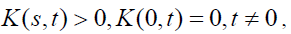it follows that If the reciprocal kernel 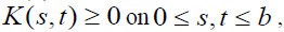is Lebesgue square integrable and continuously differentiable and if exists, then

satisfies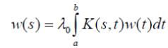 for some choice of g (t). This solution assumes that the comparison process is continuous, but it is not meaningful to compare the response during an interval of length zero with the response during a non-zero interval no matter how small it is, for then the reciprocal comparison would be unbounded. From a theoretical standpoint, one can study the problem using Lebesgue integration and allowing only one zero.

Because linear combinations of the functions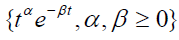

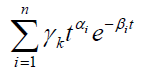
are dense in the space of bounded continuous functions C[0, b] we can approximate by linear combinations of and hence we substitute 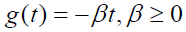in the Eigen function w (t). Later we will see that such linear combinations are dense in even more general spaces worthy of consideration in representing neural responses to stimuli. The density of neural firing is not completely analogous to the density of the rational numbers in the real number system. The rationales are countable infinite; the number of neurons is finite but large. In speaking of density in a field here, we may think of coming sufficiently close (within some prescribed bound rather than arbitrarily close).

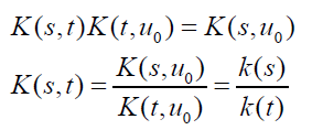
Theorem 1: K (s,t) is consistent if and only if it is separable of the form:

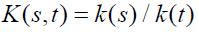
Proof: (Necessity) K (t, u₀)≠0 for some u₀∈S, otherwise K (t, u₀)=0 for all u0 would contradict K (u₀, u₀)=1 for t=u₀. Using K (s,t) K (t,u)= K (s,u), for all s, t and u, we obtain

for all and the result follows.

(Sufficiency) If K (s,t)=k (s)/k (t) holds, then it is clear that K (s,t) is consistent.

We now prove that as in the discrete case of a consistent matrix, whereby the Eigen vector is given by any normalized column of the matrix that an analogous result obtains in the continuous case.

Theorem 2:If K(s,t) is consistent, the solution of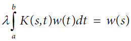 is given by

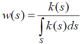
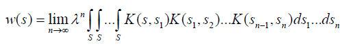
Proof: We replace 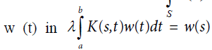by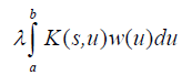 inside the integral and repeat the process n times. Passing to the limit we obtain:

Since K (s,t) is consistent, we have:

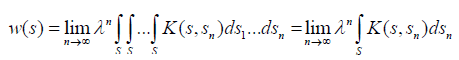
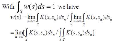
Also, because K (s, s_n) is consistent we have K (s, s_n)=k (s)/k (s_n) and

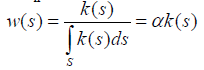
In the discrete case, the normalized Eigen vector was independent of whether or not all the elements of the pairwise comparison matrix A are multiplied by the same constant a, and thus we can replace A by aA and obtain the same Eigen vector. Generalizing this result to the continuous case we have:

This means that K is a homogeneous function of order one. Because K is a degenerate kernel, we can replace k (s) above by k (as) and obtain w (as).

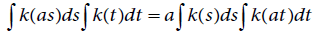
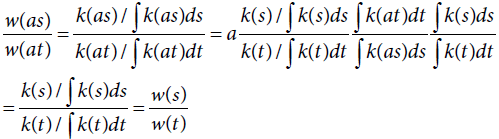
To prove that w(as) = bw(s) from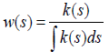 and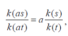 we first show that 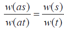Integrating both terms of 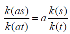first over s, we have 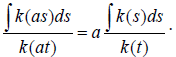Next, rearranging the terms and integrating over t, to obtain

which implies that

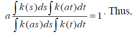
Assuming that the domain of integration is bounded or at least measurable, by integrating 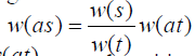over t we have 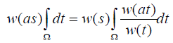and writing 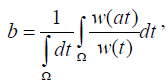we have w (as)=bw (s).

We have thus proved Theorem 3.

Theorem 3: A necessary and sufficient condition for w(s) to be an Eigen function solution of Fredholm’s equation of the second kind, with a consistent kernel that is homogeneous of order one is that it satisfy the functional equation w (as)=bw (s).

Solutions of the functional equation

W (as)=bw (s)

Real domain: If we substitute s=a^u in w (as)=bw (s)we obtain:

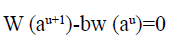
Again if we write w (a^u)=b^up (u),

P (u+1) – p (u)=0

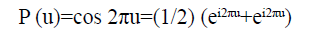
This is a periodic function of period one in the variable u (such as cos 2πu). Note that if a and s are real, then so is u which may be negative even if a and s are both assumed to be positive.

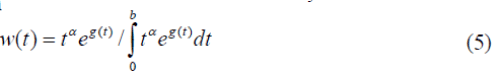
If in the last equation p (0) is not equal to 0, we can introduce C=p (0) and P (u)=p (u)/C, we have for the general response function w(s),

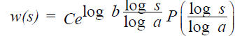
where P is also periodic of period 1 and P (0)=1. Note that C>0 only if p (0) is positive. Otherwise, if p (0)<0, C<0. As for the other solutions below, the product of two such functions is a similar function. Linear combinations of such functions are dense in the most general spaces known, e.g. like Sobolev spaces. The brain synthesizes the firing functions generated by the senses and other organs and from thought processes into a general degree of overall feeling of satisfaction and dissatisfaction. Thus we coin a new word to represent the variety and synthesis, we call the brain UNIVARIANT.

Complex domain: Note in the foregoing solution in the real domain that near zero, the exponential factor which is equal to s^{log b/log a}, "slims" w (s) if log b/log a>0 and "spreads" w (s) if log b/log a<0. Because s is the magnitude of a stimulus and cannot be negative, we do not have a problem with complex variables here as long as both a and b are real and both positive. Our solution in the complex domain has the form:

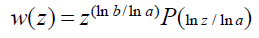
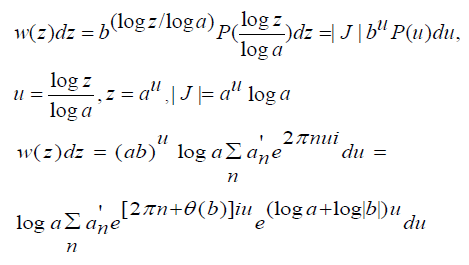
Here P (u) with u=ln z/ln a, is an arbitrary multivalued periodic function in u of period 1. Even without the multivaluedness of P, the function w (z) could be multivalued because ln b/ln a is generally a complex number. If P is single-valued and ln b/ln a turns out to be an integer or a rational number, then w (z) is a single valued or finitely multivalued function, respectively. This generally multivalued solution is obtained in a way analogous to the real case. Similarly, the general complex solution of our functional equation is given by:

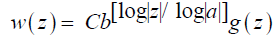
where C>0. The brackets [ ] in the above expression denotes the “closest integer from below” function and g is an arbitrary solution of g (az)=g (z).

Our solution which represents response to a force that serves as a stimulus is general and has applicability to all phenomena whose measurement is based for example, on ratio scales as in physics. When we speak of response subject to ratio scales, it is not only response of the brain to a stimulus, but also the response of any object to a force or influence to which it is subject.

We have seen that the firing function of a neuron is the product of a negative exponential and a periodic function of period one so that we have 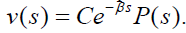Periodicity is damped by the exponential. The periodic function P (s) depends on changes in the intensity and hence the amplitude and not on the frequency. It corresponds to what is known in acoustics as periodicity pitch. At the end of each period its vibration gives rise to a firing followed by a resting period. Its periodic firing is made to happen through synapses with different other neurons whose message may sum to excitation of the given neuron or to inhibition.

The firing threshold of a neuron serves as a buffer between neurons. A stimulus received by a neuron from other neurons requires that the given neuron fire or not according to its natural response function with its natural frequency of repeated firings corresponding to the intensity of that stimulus. Thus the firings of a neuron are determined by its characteristic Eigen function, nothing else.

One form of our solution shows that there can be a part of the brain that thinks analytically, as we know there is. It is the part that is concerned with thinking and explaining. When we deal with electrical phenomena, we have no choice but to use complex variables unless we do not want to use the full information obtained. We must use complex variables to capture both: magnitude and frequency, phase or angle.

We note that we are in the habit of thinking of a stimulus in terms of its intensity represented by its modulus, which makes up half the story. However, neural response to a stimulus described in terms of real number magnitudes or in terms of its electrical character that involves amplitude and phase, must itself be expressed through electric charges involving the arithmetic of complex numbers with subtleties not encountered with real numbers.

The action of several synapses that involves the summation of many complex numbers eventually leads to (damped) periodic behavior, and because a finite sum of periodic functions is almost periodic, to an almost periodic behavior. The most compelling argument for such complexnumber periodic and hence frequency oriented, representation by synapses is that the brain can apply the Fourier transform to each term and sum the result to give us the space-time representation of the synthesis when appropriate thus making consciousness possible. Our approach assumes that each postsynaptic membrane contributes one term of a series representation and always contributes to forming that precise term. That ions arriving at the postsynaptic membrane by passing through the synaptic cleft and thus are subject to randomness, does not affect the final synthesis for that membrane to alter its contribution. Even the absence of the term contributed by a postsynaptic membrane does not have such an influence because it is but one term in a series of many such terms and does not affect the transformed and summed outcome appreciably.

Quaternions (non-commutative): In general for any quaternionic variable q we have for solution in quaternions the direct sum in which each component is single valued:

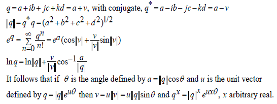
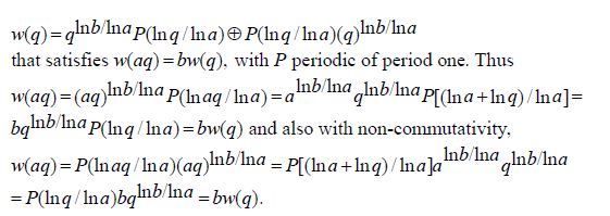
Figure 1 shows how multiplication of two quaternionic numbers is performed. To see how, as with quaternions, the idea of non-commutativity occurs in practice it can be illustrated by rotating a book 90° around a vertical axis then 90° around a horizontal axis which produces a different orientation than when the rotations are performed in the opposite order and thus the process is non-commutative. Quaternions are four dimensional, one of the dimensions, the real part describes stretch or contraction of objects and the other three, similar to complex numbers describe the angles: up or down from the horizontal level, right or left yaw and roll around a horizontal line through the center [5].

Figure 1. Quaternion multiplication.

Octonions (non-commutative and non-associative): As a vector space, the octonions are given by

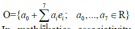
In mathematics associativity is an abundantly used property and most algebraic structures require their binary operations to be associative. On the other hand, in chemistry for example combining chemicals from compounds is a very non-associative operation. Non- associativity is well illustrated by subtracting real numbers: (7-4)-2 is different than 7-(4-2). Octonions not only do not commute but also they are non-associative. Rotation is associative but they are not commutative. The multiplication of octonions is used to describe rotations in 7 dimensions and stretch and contraction as an additional 8th dimension. String theory needs two more dimensions one for the linear string and one for time and membrane M-theory needs one more dimension than strings, that is, 11 dimensions. We have:

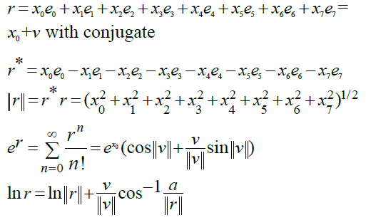
It follows that if θ is the angle defined by

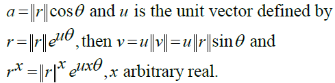
See also Figure 2 for the Fano Plane that yields the same values by moving from one node to the next with the product given by the third node in that direction.

Figure 2. Fano plane.

Not having three parts to examine associativity, our solution in the octonion domain (Figure 3) [6] as with quaternions with a and b real and positive and with P periodic of period one is given by:

Figure 3.Octonion multiplication.

First Consequence and Evidence for Validation

The laws of nature are written in the workings of our brains

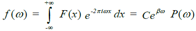
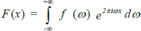
The solution of Fredholm’s equation in the real domain is defined in the frequency domain or transform domain in Fourier analysis as it is based on the flow of electric charge. We must now take its transform to derive the solution in the space-time domain. Thus our solution of Fredholm’s equation in the real domain is given as the Fourier transform,

Its inverse transform is the inverse Fourier transform of a convolution of the two factors in the product. We have:

Since our solution is a product of two factors, the inverse transform can be obtained as the convolution of two functions, the inverse Fourier transform of each of which corresponds to just one of the factors.

Now the inverse Fourier transform of e-βu is given by:

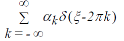
Also because a periodic function has a Fourier series expansion we have,

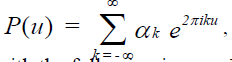
with the following inverse Fourier transform:

Now the product of the transforms of the two functions is equal to the Fourier transform of the convolution of the two functions themselves which we just obtained by taking their individual inverse transforms. We have, to within a multiplicative constant:

We have already mentioned that this solution is general and is applicable to phenomena requiring relative measurement through ratio scales. Consider the case where

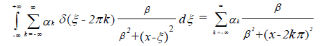
Knight [7] adopts the same kind of expression for finding the frequency response to a small fluctuation and more generally using e^i2πu instead. The inverse Fourier transform of w (u)=Ce^-βu cos 2πu, β>0 is given by:

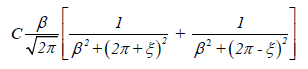
When the constants in the denominator are small relative to ξ which may be distance or whatever factor that influences a stimulus as it impacts a responder, we have C /ξ ² which describes how the inverse square laws of optics, gravitation (Newton) and electric (Coulomb) forces act. This is the same law of nature in which an object responding to a force field must decide to follow that law by comparing infinitesimal successive states through which it passes. If the stimulus is constant, the exponential factor in the general response solution is constant, and the solution in this particular case would be periodic of period one. When the distance ξ is very small, the result varies inversely with the parameter β>0.

The simple and seemingly elegant formulations in science have been questioned by scientists. LeShan and Margenau report on page 75 in their book Einstein’s Space to Van Gogh’s Sky Macmillan Publishing Co. Inc., New York 1982 that “Long after Newton proposed his inverse square law of gravitation, an irregularity in the motion of the planet Mercury was discovered. Because of a certain precession– i.e., its entire orbit seemed to revolve about one of its foci it did not exactly satisfy Newton's law. A mathematician proposed, and showed, that if the exponent 2 in Newton's law were changed ever so slightly–to something like 2.003, the precession could be accounted for. But this suggestion fell upon deaf ears: No astronomer took seriously the possibility that a basic law of nature should lack the simplicity, the elegance, the integer 2 conveyed”.

More importantly and very intriguing is the possibility that β may be very large and its effect balances off the effect of ξ. Since a stimulus often passes through a medium and arrives somewhat weaker at its response destination, the effect of the medium may be great and affects the response substantially. It seems that dark matter in space acts like such a gravitational influence medium, and moderates behavior. For example it is well-known that the outer stars of a galaxy would be driven much farther due to centrifugal force and far distance, but the effect of dark matter serves to pull these stars inwards, diminishing the overall effect of the forces countering gravitation.

Most of us think that the physical world is completely stupid and unresponsive in the way the human mind is. But apparently that is not true. Refer back to Julian Huxley’s observation about the real world. According to Huxley, all nature has a degree of awareness and solves problems. We might add that inanimate things do it in response to natural law represented by the Fourier transform. But for mental phenomena things are more complicated.

Second consequence – the weber-fechner law of psychophysics

To keep the story of the continuous case together, we decided to repeat in about a page what we have already shown before to justify the adoption of the Fundamental Scale of the AHP. It has to do with the fact that the well-known Weber-Fechner logarithmic law of response to stimuli can be obtained as a first order approximation to our Eigen function solution through series expansions of the exponential and of a periodic function of period one (for example the cosine function cos u/2π) for which we must have P (0)=1 as:

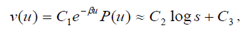
where P (u) is periodic of period 1, β = log ab,β > 0. and where β = log ab,β

The expression on the right is the well-known Weber- Fechner law of logarithmic response M = a log s + b, a ≠ 0 to a stimulus of magnitude s.

Third consequence and evidence for validation

The brain works with impulsive firings: The solution of Fredholm’s equation in the complex domain has the following Fourier Transform which leads to a linear combination of impulses. It describes which frequencies are present in the original function that is transformed. It decomposes a function into oscillatory functions. For our solution, we begin with

and the Fourier transform is given by

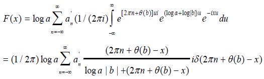
where δ (2πn+θ(b)-x) is the Dirac delta function. Actually our Fourier series is finite as the number of synapses and spines on a dendrite are finite. Our Fourier transform is written as:

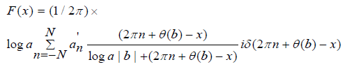
with a Dirac type of function δ involved.

When we watch birds eating from the ground, rabbits, deer and other wild animals we find that they are very jumpy and fearful and constantly look around ready to run away. Biologically we probably have similar traits that help us look out for dangers that might happen in a sequence and very quickly. Thus our attention must shift rapidly from one kind of danger to another. As a result, when we are not intentionally concentrating, our minds do not dwell long on any one thing and are jumpy. Our neurons usually are rapidly firing in expectation of sudden changes. Thus, for our improved chances of survival, we might expect the solution to our mathematical description of the brain to be impulsive, a Dirac type of distribution that adapts quickly, rather than having long segments of continuity. This is a rationalization of what we might expect in the workings of the brain.

Remark

The reciprocal property plays an important role in combining the judgments of several individuals to obtain a judgment for a group. Judgments must be combined so that the reciprocal of the synthesized judgments must be equal to the syntheses of the reciprocals of these judgments. It has been proved that the geometric mean is the unique way to do that. If the individuals are experts, they may not wish to combine their judgments but only their final outcome from a hierarchy. In that case one takes the geometric mean of the final outcomes. If the individuals have different priorities of importance their judgments (final outcomes) are raised to the power of their priorities and then the geometric mean is formed.

References

1. Saaty TL. Continuous pairwise comparisons. Fundamenta Informaticae. 2016;144(3):213-21.
2. Aczél Janos D. A short course on functional equations based upon recent applications to the social and behavioral sciences, Reidel-Kluwer, Boston. 1987;139-43.
3. Brillouet-Belluot N. On a simple linear functional equation on normed linear spaces. Ecole Centrale de Nantes, F-44 072 Nantes - cedex 03, France. 1999.
4. Shaposhnikova TO, Anderssen RS, Mikhlin SG. Integral equations, Leyden, Noordhoff. 1975;186.
5. Saaty TL. Neurons the decision makers, Part I: The firing function of a single neuron. Neural Networks. 2017;86:102-14.
6. Saaty TL. Part 2: The firings of many neurons and their density; the neural network its connections and field of firings. Neural Networks. 2017;86:115-22.
7. Knight BW. A dynamics of encoding in a population of neurons. J Gen Physiol. 1972;59:734-66.