Research Article - Journal of Agricultural Science and Botany (2020) Volume 4, Issue 3

Large Scale Agricultural Investment and a Fragile Soil Paradox in Benishangul Gumuz Regional State: Organic Carbon Stock of Broadleaf and Deciduous Forests of Combretum_Terminalia Woodlands of Benishangul Gumuz Regional State, Western and Northwestern Ethiopia.

¹Institute of Ethiopian Biodiversity, Assosa Biodiversity Center, Forest and Rangeland Biodiversity Case Team, Ethiopia

²Department of Biology, University of Bahir Dar, Ethiopia

*Corresponding Author:

Dereje Mosissa
Institute Of Ethiopian Biodiversity
Assosa Biodiversity Center
Ethiopia
Tel: +251(0)-949045964
E-mail: derament5964@gmail.com

Accepted Date: June 12, 2020

Citation: Mosissa D, Wakjira D. Large scale agricultural investment and a fragile soil paradox in Benishangul Gumuz regional state: Organic carbon stock of broadleaf and deciduous forests of Combretum ? Terminalia woodlands of Benishangul Gumuz Regional State, Western and northwestern Ethiopia. J Agric Sci Bot. 2020;4(3):1-13.

Abstract

The organic carbon stock analysis was carried out in Broadleaf and Deciduous Forests of
Benishangul Gumuz Regional State of Ethiopia with the objective of determining carbon stock
that would be found in Broadleaf and Deciduous Forests of Benishangul Gumuz Regional State
(BGRS). The assessment was conducted from 22nd September to 22nd 0ctober 2017. A total of
101 flowering plant species were sampled in 35 sample plots. Three vegetation cover types were
identified: Grassland, Open Woodland and Closed woodland. Among the different habitat types
in the area; namely: Closed Wood Land (CWL), Open Wood Land (OWL), Grass Land (GL)
and Bare Land (BL). The maximum mean Total Carbon Stock Density (TCSD) was recorded
from Closed wood land habitat with TCSD of 471 tons of carbon ha-1, followed by OWL, GL
and BL with TCSD of 375.79, 118.75 and 47.92 tons of carbon ha-1 respectively. Since the area is
located in lower altitude with low amount of rainfall per year and fire prone area, the mean total
above ground carbon stock density of the study area which is 134.94 tons of carbon ha-1 is very
low as compared to the other forest types. The anthropogenic factors (the human influence) on
the woody vegetation particularly the annual burning of the vegetation does not allow a chance
for the accumulation of carbon in the soil.

Keywords

Anthropogenic factors, Broad leaf deciduous forests, Organic carbon stock, Vegetation cover

Introduction

Vegetation in and Benishangul Gumuz Region is part of Combretum - Terminalia Broadleaved Deciduous Woodland which extends from the foot hills of western escarpment of western Ethiopia to the cost of Senegal [1,2]. This vegetation in Ethiopia was first described [3] as the Broad-leaved deciduous woodland vegetation which was later described as Combretum - Terminalia Broadleaved Deciduous Woodland Ecosystem [4,5]. This ecosystem is dominated by the woody plant species such as Lannea Fruticosa, Flueggea Virosa, Grewia Mollis, Pterocarpus Lucens, Combretum Collinum, Terminalia Laxiflora and Stereospermum Kunthianum; grasses such as Hyparrhenia Rufa and Pennisetum Thunbergii.

The amount of carbon stored in forests and different landscape components fluctuates according to spatial and temporal factors such as forest type, size, age, stand structure and associated vegetation and ecological zonation [6]. Forest management activities and associated with Silvicultural treatments are key determinants of forest carbon dynamics.

The study area belongs to high fire frequency zone, which occurs across sub Saharan Africa from Senegal to the western Ethiopian escarpment, and also penetrates into the highlands along the deep river valleys [7]. The influence of elevated temperatures at lower altitudes and rainfall is known to have direct impact on the intensity and frequency of fire in the area. The plants in this vegetation have, over time, developed adaptive mechanisms and traits that allow them either to survive fire, to germinate after the heat shock or to regenerate after a fire episode. The selective pressure of fire on the plant communities has produced plant species, which are fire resistant, or pyrophytes [8]. The incidence of annual fire for a long period of time in the area shows many adaptations of plants both to burning and its impact on soil properties [7,9].

The rationale for this study was to collect data and information, is to serve as a statistically valid estimation of forest biomass and carbon stock within each habitat types in the given area site. The assessment was conducted from 22^nd September to 22^nd October, 2017.

Materials and Methods

Location description

The assessment was conducted in western and northwestern Ethiopia (In Benishangul Gumuz Regional State), located between latitudes 09°17'N and 12° 'N and longitudes 34°10' and 37°04' E. The capital of the region (Asosa) is located at a distance of 687 km from the capital city of Ethiopia i.e Addis Ababa. The administrative region of the study area is bordered by Amhara National Regional State to the north, Oromiya National Regional State to the east and south, and the Republic of the Sudan to the west. The topography of the area is characterized by undulating elevation which decreases gradually toward the western part to an average altitude of 500 m along the Ethiopia -Sudanese border (Figure 1).

Figure 1. Topographical map with Benishangul Gumuz National Regional State outlined in black. Altitude in meters is given in the legend (Source: modified from Tesfaye Awas 2009).

Geology and soils

The geology of the area is mainly outcrops of very old Precambrian rocks that underlay all the other rock types in Ethiopia [10] (Figure 2). Poly-deformed and Poly-metamorphosed crystalline rocks overlay the Precambrian rocks, and is one of the areas in Ethiopia where these rocks are exposed [11]. These rocks hold most of the mineral deposits, particularly gold but also copper, lead, and zinc. In addition, there is an important occurrence of marble, which are to some extent utilized. Nitisols and Acrisols are the predominant soil types in the region (BGNRS) [12].

Figure 2. Partial view of the Geological map of Benishangul Gumuz Region Ethiopia (Source: modified from EIGS, 1996).

Climate

The climate of the region is characterized by a single maximum rainfall that runs from April/May to October/November. The average annual precipitation varies from 900 mm to 1500 mm. The mean monthly minimum and maximum temperature varies from 14°C to 18°C and 27°C to 35°C, respectively (Figure 3).

Figure 3. Climate diagram of BGRS (Data source: NMA, 2018).

Approach and methodology for the biomass assessment

Inventory and soil sampling: An initial inventory and assessment of the plots was conducted prior to the destructive sampling, this inventory and soil sampling was carried out by a team of experts. The placement of the plots followed mostly transects that crossed through the various habitats in the reservoir and a stratified sampling technique was used, representing 45.71% Grassland, 28.57% open woodland and 22.86% closed woodland.

Soil samples were collected during the inventory where a 30 cm mini-pit was dug and utilised to collect information such as soil texture, colour, moisture, structure, roots, micro-relief, etc. For the soil sampling the method followed was, standardised description of the soil subsequently, four hits in four corners of the plot were dug to a depth of 30 cm, accordingly 500 g of soil sample was collected from each pit. These samples were mixed on a plastic sheet; all stones and wood debris were then removed, ensuring that only organic matter is remaining and 500 g were bagged, ensuring adequate labelling with the plot identification code/number, and sample number. Follow-up was made to air dry the samples under shade in order not to prevent the soil samples from being spoiled. The soil samples were divided in to two subsamples of approximately half the amount and one of the samples was sent to the laboratory for analysis, and the other stored as a duplicate in case of loss or any additional analysis deemed necessary. In parallel, a cylindrical core sampler with 5 cm internal diameter and 5 cm height having a volume of 98.17 cm3 was used to collect soil sample for bulk density analysis. This was collected from each plot.

The objectives of this sub-task were the following:

• Collection of recent vegetation data in order to increase knowledge about the regions current vegetation data and inform the future investment plan;

• Conduct the soil sampling in order to be able to quantify the soil organic carbon in the area under study.

• Conduct destructive sampling of the Above Ground Biomass (AGB), (Trees, Shrubs, Herbs and Grass ) and Estimate the carbon stock existing in the above and below ground biomass within the different habitats in the study area.

Measurement of forest carbon pools: Three forest carbon pools including above ground (trees, saplings and leaf litter, herb and grass), belowground biomass, and soil organic carbon pools were measured. The details of field measurement techniques and methods for estimating forest carbon stock for these different pools are described in the following sections.

Tree inventory methodology

Within the transect lines the distance between plots was one km and the distance between two parallel transect lines were 10 km. Plot’s geographical coordinates and other data are presented in annex 1. The first plot in a transect was placed randomly. According to a study [13], sampling design for the collection of AGB data should be a multipurpose one in order to realize efficiencies in data collection and minimize costs. Therefore, the plots that were used to take measurements for AGB biomass estimation were also used for biodiversity (vegetation) and other data. The sampling plots of regular shape of dimensions 10 x 10 m and sub plots of four 1 x 1 m, were used for woody and herbaceous respectively.

After deciding the plot, the corners of the plot, were marked and the corresponding coordinates/GPS waypoints were taken. Then from each plot, the following information was systematically collected from each individual tree:

• Species (or genus),

• Height (measured with clinometers),

• Canopy cover,

• Diameter At Breast Height (DBH),

• Diameter At Stump Height (DSH)

On top of the above records for individual trees, the presence of all trees, shrubs, herbs, herbaceous climbers and grass species that occurred within the plot were recorded. In addition, general plot description on physical aspects, including leaf litter coverage, altitude, slope and aspect were collected. Status of regeneration and anthropogenic disturbances were also recorded for each plot. Accompanying photographs and coordinates/GPS readings of each corner of the plots were recorded, in order to ensure a thorough documentation of the plot prior to the destructive sampling. Information on location (District, Kebele and locality names) where the plot is located was recorded. This information was used to complement the data from earlier studies, and also inform the destructive sampling survey plan.

Soil sampling

According to a study [14,15], in order to obtain an accurate inventory of organic carbon stocks in the soil, the following three variables were measured: soil depth to which carbon is accounted (usually 30 cm), soil bulk density which is calculated from an oven-dry weight of soil from a known volume of sampled material and concentrations of organic carbon.

Soil samples were collected during the inventory where a 30 cm mini-pit was dug and utilised to collect information such as soil texture, colour, moisture, structure, roots, micro-relief, etc. For the soil sampling the method followed was, standardised description of the soil [16], subsequently, four hits in four corners of the plot were dug to a depth of 30 cm, accordingly 500 g of soil sample was collected from each pit. These samples were mixed on a plastic sheet; all stones and wood debris were then removed, ensuring that only organic matter is remaining and 500 g were bagged, ensuring adequate labelling with the plot identification code/number, and sample number. Follow-up was made to air dry the samples under shade in order not to prevent the soil samples from being spoiled. The soil samples were divided in to two subsamples of approximately half the amount and one of the samples was sent to the laboratory for analysis, and the other stored as a duplicate in case of loss or any additional analysis deemed necessary. In parallel, a cylindrical core sampler with 5 cm internal diameter and 5 cm height having a volume of 98.17 cm³ was used to collect soil sample for bulk density analysis. This was collected from each plot.

Destructive vegetation sampling

The carbon stock assessment of broadleaf deciduous forested areas of Benishangul Gumuz Regional State (BGRS) was conducted using destructive vegetation sampling in order to quantify the carbon sequestered by various natural habitats. The extent of the area covered was 1680 km²; in order to follow the sampling requirements set out by the proposal, a total of 35 plots of 10 x 10 m were assessed. These plots were distributed within the stratified habitats in the area under study. The information gathered during the inventory facilitated the choice of the plots to be destructively sampled. All trees were destructively sampled in order to determine their AGB.

The destructive vegetation sampling was conducted by a team of experts, technical assistants and labourers. Where two experienced foresters, one botanist who can readily identify all tree, herbaceous and grass species and two Ecologists were team members, with one technical assistant which is a chainsaw expert. Labourers were hired locally in order to assist the team with orienteering and helping with identification of the accessible sites.

Plot preparation

Once arrived on the plot, a rapid assessment was done based on the prior information gathered. Trees that are to be felled were identified and appropriate set-up initiated for each tree (e.g. lying of tarps, lying out of sampling bags, etc). During the preparations the leaf litter, understory and dead wood sampling were carried out. Destructive sampling took place once the plot preparation is complete (Table 1). Each of the following elements was collected within the plot boundaries following the methodologies specific to each:

Table 1. A summary table of measurements taken in the field.

• Trees (DBH > 5 cm)

• Shrubs (< 5 cm)

• Leaf litter, non-woody material, and saplings (DBH < 5 cm)

• Dead wood and stumps.

Trees (DBH > 5 cm): Once the plot preparation is complete, trees are felled. Only one tree was felled at a time to avoid contamination between specimens. Once the tree is down, due to the diverse nature of the different parts of trees (Figure 4), different sampling methods was utilised for different sections. All trees above and equal to 5 cm in diameter at breast height (DBH) within sample plots were measured and recorded on the data sheet.

Figure 4. Different sections of a tree.

The trunk: As the tree was down, the length of a tree from the stump to the top of the crown, the length of the trunk from the stump to the first main brunch and the height and diameter of the stump was measured in meters. The diameter of the trunk was measured every one meter top and bottom. Weight measurements for the trunk ( > 20 cm and between 10 cm and 20 cm diameter) was taken after the tree is being cut every one meter and when it becomes difficult to cut at one meter then length was noted carefully, cut at a manageable length and weighed. Main branches ( > 20 cm and between 10 cm and 20 cm diameter) were also measured the same way as that trunk was measured.

The crown: The crown is sectioned into thick branches, thin branches, leaves and other soft fractions. Based on the information gathered from the field inventory the specific size thresholds were defined and have not been altered, throughout the entire destructive sampling. Soon after the tree was down, several length and weight measurements were taken from different parts of the tree. For thick branches, thin branches, leaves & fruits total fresh weight were measured.

The three sections of the crown were;

• Thick branches (basal diameter between 4 cm and 10 cm): these are gathered together and weighed as a whole;

• All thin branches with a basal diameter between 2 cm and 4 cm were gathered together, and fresh/ wet weight recorded as a whole.

• Leaves and other soft fractions (e.g. fruit and twigs): the soft fraction was collected and weighed as a whole. And a minimum of 200 g of leaves and twigs was collected and weighed.

A minimum of three samples (whenever possible), were bagged, fresh/wet weight was taken and labelled with the relevant identification details (e.g. plot number, species name, tree number, and sample number) for thick & thin branches and also for leaves. Woody subsamples were taken with a minimum of 10 cm in length (whenever possible).

Wood density: Due to the total weight and volume of the trunk and main branches, their dry weight is estimated from the volume of each 1 m section and the wood density of the particular species. In order to determine the tree density, a minimum of three trees of varying DBH per species (whenever possible), cross-sectional discs of 30 mm to 50 mm in thickness were sawn from the main trunk, main branch and other branches with > 10 cm are bagged and weighed. Each bag was labelled with plot code, tree identification number, and sample weight and sample number [17].

Shrubs: Shrubs were sampled destructively in a similar manner to trees – by separating the soft fraction (leaves and fruiting bodies) from the woody biomass. Each section is then weighed, and a minimum of three samples bagged, weighed and labelled with the relevant identification details (e.g. plot number, tree number and sample number).

Leaf litter, non-woody material, and saplings: To determine the biomass of leaf litter, grasses, shrubs and saplings (DBH < 5 cm), four 1 x 1 m plots were sampled. The plots were placed at each corner, (Figure 5). All plant biomass from these sub –plots (1 m x 1 m) was carefully collected, ensuring that the leaf litter and other small dead organic matter (e.g. twigs) were separated from the non-woody and woody live biomass (e.g. grass, saplings, lianas) and was, placed in a plastic bag and fresh weight was taken on site using a balance. For each of these subplot and sub-categories, 200 g sub sample was bagged, fresh weighed and labelled with plot number then, the sample was oven-dried in the laboratory in a conventional oven at 70°C to a constant weight, which enable calculation of the total dry mass.

Figure 5. Sampling plot (10 x 10 meters – Black Square) for trees and shrubs, with nested plots (1 x 1 meter - green squares) for grasses, saplings and litter.

Dead wood: Dead wood can be one of the most difficult biomass pools to assess due to its variability. Due to the nature of the habitats, the common yearly burning practices in the area, and the size of the plots, the quantity of dead wood that will be encountered is most likely limited. Nevertheless, a methodology for dead wood sampling was the following.

The first category of large dead wood is stumps and other standing dead wood. If dead tree only consists or a trunk or stump; simple measurement of its basal and top diameter can be taken, along with the height for a volume estimation. Disks for wood density measurements were also taken for each individual dead tree. However, whenever dead tree is in its early stages of decomposition, and still presents branches of varying sizes, it was sectioned into the different woody sections (e.g. trunk, branches, stump), and proceed similarly to trees. For fallen dead wood, there were two categories – larger logs or branches (diameter > 10 cm) and small dead wood. The small diameter was dealt within the leaf litter. For the larger fallen wood, the total length and diameter at both ends is recorded, and a disk sample collected in order to determine the wood density (similar to logs).

Whenever, standing trees or fallen logs have cavities or are hollow, the appropriate dimensions were taken in order to estimate the volume of the cavity. This cavity volume will have to be subtracted from the total calculated volume [15].

Below Ground Biomass (BGB) Estimation: The belowground organic pool includes soil carbon, roots and microbial biomass. However, the below ground tree biomass (roots) is difficult and in most cases it is considered through a relationship to above ground biomass. For this study, from the total belowground organic pool, only below-ground biomass (tree roots) and soil carbon were considered.

Laboratory methodology

All of the bagged materials (soil during the inventory phase, biomass during the destructive sampling phase) were taken to Assosa, Benishangul Gumze Regional National Soil laboratory, for processing, following the methods listed below (Table 1).

Above ground biomass: All samples bagged and submitted to the laboratory were dried in order to determine the dry weight of each section (e.g. trunk, branch, leaves, etc.). The drying process took place in drying ovens set at 105°C for the wood, and 70°C for leaves, leaf litter and herbaceous species. The drying process was considered complete when the weight of the sample remains constant (approx. 2 days to 7 days, depending on the nature and dimensions of sample). These weights represent the dry biomass weight of each respective sample (B_dry).

Wood density measurement: For certain sections (e.g. trunk, main branches and other branches with diameter > 10 cm and dead wood) discs were collected in order to determine wood density for specific tree species / dead trees. The procedure for this - water replacement method - is following [18] is described below:

A graduated container large enough to accommodate the wood sample was filled with water and placed on a scale. The wood sample, which has previously been saturated with water (48 h immersion), is then lowered into the container; care has been taken to prevent that the displaced water not flow over the sides of the container. The volume of the wood sample (vi) is equal to the volume of the displaced water. According to the same procedure as the other samples.

Density is then calculated as:

where ρi density

mi = dry weight of the wood sample

Vi = volume of the wood sample

This is repeated for each disk; for live trees, an average density was calculated per species. However, for dead trees, the value was used only for the individual specimens.

Soil Organic carbon analysis: Soil Organic Carbon (SOC) was estimated from the sub-samples taken in the field from each plot. While there are a number of methods being used or developed at the present time for SOC, the wet digestion method devised by [19] remains useful if the necessary correction factors are applied. The composite samples collected from each plot was air-dried, crushed, and passed through a 2 mm sieve in the laboratory. Most stones will be removed from the soil in the field. Any stones left after 2 mm sieving will be kept separately but not analysed.

The principal analysis from a soil sample at each site will be for Soil Organic Carbon [SOC], and the air dried soil samples were subjected to chemical analysis using the method originally developed [19]. The approved methods a wet digestion using a N-Potassium dichromate [K₂Cr₂O₇] solution and a concentrated sulphuric acid [H₂SO₄]. The procedure is as follows: A weighted sample of air dried soil is placed in a 500 ml flask; N-potassium dichromate and then sulphuric acid were added, and digested for 30 min. De-ionised water is then added and the solution left to stand for one hour. 85% Ortho-phosphoric acid (H₃PO₄) and a Diphenylamine Sulfonate indicator were added, and the solution is back-titrated with 0.5 N-Ferrous Ammonium (0.5 N Di Ammonium Ferrous Sulphate (Mohr’s Salt) until the colour change occurred noted. The volume of the Ferrous Ammonium Sulphate is registered and a blank titration made in similar manner. The calculation of % organic carbon of a given sample ( pi %OC ) is made using the following equation:

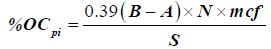
Where B is the volume (mL) of ferrous sulphate solution required for blank titration

A=is the volume (mL) of ferrous sulphate solution required for sample titration

N=is the normality (N) of ferrous sulphate solution

Mcf=is the moisture correction factor

S=is the weight of the soil sample (g)

With this method, about 77% of the carbon is oxidized by potassium dichromate, suggesting that a correction factor of 100/77=1.3 needs to be applied in order to get a more accurate estimation of the carbon.

Soil bulk density: For soil bulk density analysis, a cylindrical core sampler with 5 cm internal diameter and 5 cm height was used in order to collect a soil sample for the calculation of the bulk density.

Soil bulk density, which is calculated as the oven dried weight of soil divided by its volume is calculated using the following equation [20].

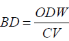
Where: BD=Bulk density (gm/cm³), ODW=Oven dried weight of soil (gm.) and CV=Core volume (cm³).

If a large quantity of rocks is found in the sample, a correction for these will be used:

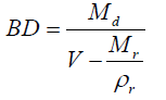
There Mr as the mass of the rock fraction ρr as the rock fraction density (set at 2.6 g/cm³).

Data on bulk density and carbon concentrations were used to compute amounts of carbon per unit area. Then the amount of soil organic carbon per unit area was calculated as:

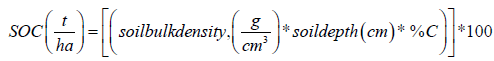
In this equation % C must be expressed as a decimal fraction; for example, 2.2% C is expressed as 0.022 [15].

Data analysis

The data analysis creates the link between the information collected on the field (e.g. wet weights, tree characteristics) and the measures obtained in the laboratory analysis (e.g. dry weights, bulk density). A comprehensive summary table of all the data collected is presented in Table 1.

Above-ground biomass analysis: The different categories of biomass were dealt separately, though the method is similar: The procedure followed that; first determining the AGB of the sampled plot for the category (either 10 x 10 plot for trees, shrubs and dead trees, or 1x1 m plots for aboveground nonwoody material, saplings and leaf litter), and then extrapolating to a per hectare basis using an expansion factor. A brief summary for each is presented below:

• Tree Biomass (AGB_trees) – the tree biomass were first determined on a plot basis, where the total tree biomass of a given plot is the sum of the biomass of every tree encountered in the plots, including woody and non-woody sections. This value was then extrapolated into a per hectare basis using an expansion factor.

• Shrubs Biomass (AGB_shrubs) - similarly to the tree biomass, the shrub biomass for any given plot was the sum of the biomass of each shrub encountered. This is then extrapolated into a per hectare basis using an expansion factor.

• Dead wood (AGB_DW) - similarly to the tree biomass, the dead wood biomass for any given plot is the sum of the biomass of all dead wood encountered. This is then extrapolated into a per hectare basis using an expansion factor.

• Aboveground non woody material and saplings (DBH < 5 cm) (AGB_NW) – the average weight of 1 m² was calculated per plot (using the 4 samples), and then extrapolated to per plot and a per hectare basis.

• Leaf litter (AGB_LL) – the average weight of 1 m² was calculated per plot (using the 4 samples), and then extrapolated into a per hectare basis.

Tree biomass (AGB_trees): Individual tree biomass is calculated one of two ways:

• For trees that are destructively sampled: summing the estimated dry weight of each of their sections. The larger woody sections will be estimated based on volume, and for the smaller sections, including branches with basal diameters of less than 10 cm and the soft fraction, using moisture based estimates.

Woody biomass: The woody biomass is represented in two categories:

• Trunks and main branches < 20 cm: these require to extrapolate the dry weight through their volume

• Branches of less than 10 cm and > 4 cm basal diameters: the dry weight was computed using the wet weight to dry weight ratio.

Trunks and main branches: Using Smalian’s Formula, the volume of each section of the branches and trunks of each of the sampled trees can be calculated as:

Where V=Volume

L=Length of the trunk

D₁=Diameter of the narrow end of the trunk

D₂=Diameter of the large end of the trunk

Once the volume is determined for each section, the mass can be calculated using the species-specific density, such as:

For each tree, the total mass of its large woody fraction will be the sum of the estimated mass of all the trunk and main branches sections

Soft fraction and small branch biomass: For each sample, a dry to wet weight ratio (or moisture content) (X_i) was developed as:

where: X_i the wet to dry ratio of the sample

B_wet the wet weight of the sample

B_dry the dry weight of the sample

This value was then used to reciprocally calculate the dry weight of each sample, using the Bwet weighed on the field for the particular section (e.g. small branch, leaves).

Shrubs: Determining the biomass of each shrub will be similar to that of the non-woody sections of each tree: determining the dry to wet ratio for each section using the sample, and then using it to determine the total dry weight of the section weighed in the field. The biomass of each shrub is the sum of the dry weight of each of its sections.

Dead wood: Dead wood (excluding small branches which are collected with leaf litter – will be treated as the branches and trunks – by determining the wood density using the disk samples) and the volume based on the measurements gathered on the field (using Smalian’s formula. By adding the estimated biomass of each sampled dead wood per plot will determine the AGBDW for that plot.

Leaf litter, above-ground non-woody material and Saplings: This portion was treated in a similar fashion as the non-woody sections of the trees using a wet to dry biomass ratio of the sample returned to the laboratory. Then it was used to calculate the dry weight of each plot sample.

This is to be done separately for the leaf litter (including small dead wood), and for all the live above-ground material (i.e. grasses, sapling and lianas).

Expansion factor: The unit for each of the values above was expressed in a mass per unit area. In order to homogenise the unit area (hectares), each section had its AGB multiplied by an expansion factor (E) (Table 2).

Table 2. An expansion factor (E).

Correction factors used are presented in the above table. For the mass unit, it is vital to ensure that the mass units are consistent between sections, prior to determining the total volume (i.e. g, kg, or t).

Above-ground carbon pools: Once the AGB of each section is determined, the carbon fraction must be determined. This study used the standard set by IPCC (Intergovernmental Panel On Climate Change) guidelines for National Greenhouse Gas Inventories [21] and the Good Practice Guidance for Land Use, Land-Use Change and Forestry [22] in order to calculate the average carbon pool per habitat. The average carbon fraction of aboveground live biomass and dead wood is set at 47%, while for leaf litter (CLL) it is set at 37%.Therefore, for all the carbon pools listed above, the AGB to carbon relationship is:

C_i = 0.47×AGB_i where: the designating the category of the live biomass (e.g. trees, shrubs, non-woody) or dead wood

C_LL = 0.37× AGB_LL The above-ground carbon pool (C_plot, unit: tC.ha^-1) is then calculated as:

C_plot=C_trees+ C_shrubs+ C_DW+ C_NW+ C_LL

The carbon pool per hectare for a given habitat () can then be calculated by averaging the carbon pool value of all the plots within a given habitat). Theseaverages were used to compute the estimated above-ground carbon stock of each habitat within the study area (Figure 6).

Figure 6. Flow chart of how the AGB for each biomass section (determines an average carbon stock per habitat (C_i; unit: tC.ha^-1).

Below-ground carbon

Soil organic carbon: For each plot, the amount of Soil Organic Carbon per area (SOC_i) is calculated as:

where: BD = the bulk density of the soil

Depth = the depth of the soil stratum

% OC_pi = Fraction of organic carbon in sample (%)

As it is with the other carbon pools, it is crucial to verify the units; It is expressed and ensure adequate conversion (e.g. g.cm² to t.ha^-1).

From the estimates of each plot, an average value (with associated errors) was calculated per habitat. This average was then used to compute the estimated soil carbon stock of each habitat within the study area (Figure 7).

Figure 7. Flow chart of the soil carbon analysis procedure, from collection of samples to determining an average carbon stock per habitat (C_i; unit: tC.ha^-1).

Below ground biomass (BGB) estimation: For below ground biomass a standard root: shoot ratios (R) which is a 1:5 root to shot ration commonly used parameter in converting standing volumes of tree into total carbon stocks [23]. Therefore, the following equation was used to estimate Below Ground Biomass (BGB):

BGB=ABG * R

Where: BGB=Below Ground Biomass,

ABG=Above Ground Biomass and

R=root to shoot ratio (0.2).

Determination of the total carbon stock (TCS) per hectare: The above-ground biomass carbon contained in a given habitat is calculated as the product of the average AGB carbon per hectare (C_h – tonnes per hectare) of that habitat and the area of the habitat. Similarly, the total soil carbon of a given habitat is calculated as the product of the average SOC of that habitat and the area of the habitat.

The Total Estimated Carbon Stock (TCS) which is the sum of all carbon stocks in all carbon pools and expressed as tons per hectare was calculated by adding all the carbon stock densities of the individual carbon pools from the sum of each habitats of the study area.

TCS is, therefore, calculated by using the following formula:

Carbon stock density for all pools (tons of C ha^-1)

C_AGB=Carbon in above ground biomass (tons of C ha^-1)

C_BGB=Carbon in below ground biomass (tons of C ha^-1)

C_Lit=Carbon in litter (tons of C ha^-1)

S_OC=Soil organic carbon (tons of C ha^-1)

Result and Discussion

Vegetation

During the assessment, a total of 101 flowering plant species were sampled (Annex 2 and Table 3) in 35 sample plots. Three habitat types were identified: They were; Grassland, Open Woodland and Closed woodland. Grassland habitat type is created mainly by removal of trees from closed woodland as part of vegetation clearing program from reservoir area and anthropogenic factors such as regular fire etc. The trees were cut and moved out from the reservoir area and pilled outside to be inundated area shows one of the sites where the wood is pilled.

Table 3. Habit characteristics of plants encountered in the study area.

This vegetation type is known to have an annual forest fire where every year the tall grass which is dominant burns and there is a clear scar on trees showing that burning was evident. Some of the trees have been observed to have developed adaption to fire and their bark thickened. This anthropogenic influence is known to exist for a very long time.

This vegetation type is currently seen as an area of cultivated land expansion, homes of Frankincense, bamboo, and the wildlife and sources of the wildlife food and feed/substrate. The area also provides wood for construction and domestic fuel.

Above ground biomass (AGB) estimation

Above ground herbaceous: The mean herbaceous above ground carbon stock of the reservoir area was 3.96 tons of Carbon ha^-1. The maximum herbaceous above ground carbon per plot was recorded from plot one with 17.68 tons of Carbon ha^-1 which is an open woodland (Table 4) which obviously encourages a herbaceous growth because of low tree density. The minimum was recorded from plot four with zero tons of Carbon ha^-1 (Table 5).

Table 4 . Plots by habitat type, their percentage and average carbon density.

Table 5. Biomass and carbon stock within different carbon pools.

Above ground tree and shrub biomass: The average above ground carbon stock for trees and shrub of the reservoir was 290.41 tons of Carbon ha^-1, which includes the soft fractions, twigs & fruits, leaves, small branches, big branches, main branches and trunks. Plots in the closed woodland had mean carbon stock of 471.00 tons of c/ha, while plots in open woodland had 375.79 tons of carbon ha^-1 for trees and shrubs (woody biomass).The result showed that the maximum and minimum carbon per plot was recorded from plot 17 and 28, with 1178.28 and 59.99 tons of Carbon ha^-1, respectively. The result of plot 17 is far high from the others; because of that it is a very dense forest with big trees and trees with high wood density. As it was clearly stated [6], big trees represent important proportion of the forest biomass; hence data are skewed towards big trees.

Above ground Litter biomass: The mean litter carbon density of the reservoir was 0.44 tons of carbon ha^-1 and the maximum litter carbon stock density per plot were recorded from plot 23 followed by 5, 20 and 32 with 1.83, 1.69, 1.39 and 0.92 tons of carbon ha^-1, respectively. The minimum litter carbon density was recorded from plot one, four, six and seven with no litter fall at all and preceded by plot ten with 0.05 tons of carbon ha^-1 (Table 5). The Litter biomass and carbon stock by habitat type showed a similar trend as that of woody biomass, where the maximum value recorded from closed woodland followed by open woodland and grass land with 0.60, 0.45 and 0.38 tons of carbon ha^-1 respectively. The litter is high in closed woodland as there are many trees which can shade much leaves than the open woodland and grassland habitat types.

Total above ground biomass: The total above ground biomass and carbon stock per ha is the sum of all the above ground pools which are: herbaceous carbon stock, trees and shrub carbon stock (leaves & twigs, thin branches, thick branches, main branches and trunk) and litter carbon stock. Therefore, the total average above ground biomass and carbon stock of the study area was 290.41 tons/ha biomass and 136.37 tons carbon/ha, respectively.

Below ground biomass (BGB): As that of the above ground biomass, below ground biomass showed similar trend in terms of plots recorded, the maximum and minimum values, since it is a function of the aboveground biomass. The maximum and minimum below ground carbon per plot were recorded from plot 17 and 4, respectively with 236.16 and zero tons of Carbon ha^-1 (Table 5). Whereas, the mean below ground carbon stock of the reservoir was 27.30 tons of Carbon ha^-1.

The result from soil laboratory analysis for the percentage of soil organic carbon showed that, the mean soil organic carbon of the reservoir was 2.6% which ranged from 1.32% for plot four to the maximum of 4.06% for plot 34. The soil bulk density analysis showed a range from 0.708 g cm^-3 for plot 15 gcm^-3 to 1.736 gcm^-3 for plot six; whereas, the average soil bulk density was 1.39 gcm^-3 for the whole reservoir. The result showed that, the mean soil carbon stock density was 107.2 tons of carbon ha^-1, while the maximum and the minimum were recorded from plot 30 and 4, respectively with soil carbon stock density 162.75 tons and 47.92 tons of Carbon ha^-1 (Table 5).

Average carbon stock density by plot and habitat type: The average Total Carbon Stock Density (TCSD) of the reservoir was 270.98 tons of carbon ha^-1. While the highest TCSD was recorded from plot 17 which is 1520.44 tons of carbon ha^-1, followed by plot 20, 22 and 32 with 744.89, 522.78 and 461.19 tons of carbon ha^-1, respectively; while the minimum value was recorded from plot 4 with 47.92 tons of carbon ha^-1.

The low contribution of below ground and litter biomass seems to be because of fire incidences in the area. In the study area Benishangul Gumuz Regional State (BGRS), the bush fires occur between December and February. The combination of climatic factors, such as maximum temperature and low humidity during this period contribute to the increase in the probability of fire. Fire has played an important role over evolutionary, historical, and ecological time influencing their composition, physiognomy; and fuel availability and the relationship between fire and the plant and the associated wildlife is the result of mutual compromise. Thus, it is possible to suggest that the vegetation provides certain properties to the ecosystem that condition the fire regime; and the fire regime determines in part, the maintenance, regression, or succession of plant and animal communities. The burnt grass and herbaceous species restart at their rhizomes, bases and bulbs, which are normally subterranean [18].

The elevated temperatures at lower altitudes, increases the intensity and the frequency of woodland fire. Burning reduces the organic carbon content of the soil and leads to accumulation of mineral salts, which increase base saturation and pH. Evapotranspiration under elevated temperature and low rainfall also increases salt accumulation. On the other hand, altitude was positively correlated with an increase in Cation Exchange Capacity in the top soil, exchangeable magnesium in the top soil, organic carbon and total nitrogen. At higher altitude absence of fire allows accumulation of organic carbon and nitrogen, which increases the Cation Exchange Capacity of the soil. This facilitates absorption and accumulation of mineral salts in the plant tissue. Several studies [7,24] on woodland fire have come up with such findings [12].

Among the different habitat types in the reservoir namely, Closed Wood Land (CWL), Open Wood Land (OWL), Grass Land (GL) and Bare Land (BL); the maximum TCSD was recorded from Closed wood land habitat with TCSD of 470.83 tons of carbon ha^-1, followed by OWL, GL and BL with TCSD of 377.79, 118.66 tons and 47.92 tons of carbon ha^-1, respectively (Figure 8). The result shows that closed woodland even with comparatively low number of sample plots had the highest carbon stock density per ha^-1 while the bare land and Grassland had lower carbon stock density. Though, the result is higher than the average value for tropical dry forests according to IPCC, 2006; it is less than other similar forest studied in Ethiopia which reach up to 589.24 ton ha^-1 carbon [25].

Figure 8. Carbon stock in different habitat types in the reservoir namely, Closed Wood Land (CWL), Open Wood Land (OWL), Grass Land (GL) and Bare Land (BL).

Conclusion

Forest biomass and carbon accumulation are governed and influenced by several factors such as climate, type of species and anthropogenic factors. Apart from these, site specific conditions such as annual forest fire, altitude, slope, aspect and other environmental variables play an important role on forest biomass accumulation and carbon dynamics. Since the reservoirs is located in lower altitude with low amount of rainfall per year and in fire prone area, the mean total above ground carbon stock density of the reservoir which is 138 tons of carbon ha^-1 is very low as compared to the other forest types. The anthropogenic factors (the human influence) on the woody vegetation particularly the annual burning of the vegetation does not allow a chance of the accumulation of carbon in the soil. The litter carbon (0.44 tons of carbon ha^-1) among the various carbon pools. There were three vegetation cover types identified (Grassland, Open Woodland and Closed woodland). The grassland and the woodland habitat type were clearly the result of human activity and mainly the current removal of closed and open wood land. The study concludes that the amount of carbon stored in different habitats varies considerably depending on forest conditions (age and site conditions).

Author Contributions

The lead author Dereje Mosissa was the principal investigator for the research and took the study from inception, through to fieldwork, data management/analysis, drafting, and proofing of the manuscript. Dawit Wakjira provided technical inputs into cross interpretation, editing, and proofing of the manuscript.

Funding

This research received no external funding.

Acknowledgments

The authors would like to thank the support from the agriculture officials and farmers who participated in the study; Benishangul Gumuz Regions’ Environment Land and Investment Bureau, Assosa University and Assosa Biodiversity Center for their technical and financial support in analysis and writing of this article. Finally the Author would like to acknowledge Tesfaye Awas (PhD) for his special supports in suggesting methods for organic carbon stock analysis.

Conflicts of Interest

The authors declare no conflict of interest

References

1. Awas T. Plant Diversity in western Ethiopia: Ecology, ethno botany and conservation. University of Oslo, Norway 2007.
2. White F. The Vegetation of Africa. A descriptive memoir to accompany the UNESCO/AETFAT/UNSO vegetation map of Africa. Natural Resources Research. 1983;20:1-356
3. Rodolfo Pichi-sermolli EG. Una carta geobotanica dell’Africa Orientale (Eritrea, Etiopia, Somalia). Webbia. 1957;13:15-132.
4. Anonymous. Conservation strategies of Ethiopia, Addis Ababa 1991.
5. Awas T, Gashaw M, Tesfaye G, et al. Ecosystems of Ethiopia, IBCR, Addis Ababa 2003.
6. Jun Ma, Yuanman Hu, Rencang Bu, et al. Predicting impacts of climate change on the aboveground carbon sequestration rate of a temperate forest in North-eastern China. PLoS one. 2014;9(4):e96157.
7. Jensen M, Friis I. Fire regimes, floristic diversity, life forms and biomass in wooded grassland, woodland and dry forest at Gambella, western Ethiopia. Biologiske Skrifter. 2001;54:349-87.
8. Kunholtz-Lordat G. La terreincendiée, Essaid’agronomie comparée. La MaisonCarrée Nimes.1938;361.
9. Menassie Gashaw, Michelsen A, Friis I, et al. Post-fire regeneration strategies and tree bark resistance to heatingin frequently burning tropical savanna woodlands and grasslands in Ethiopia. Nordic Journal of Botany. 2002;22:19-33.
10. Mohr Paul A. The Geology of Ethiopia. University College of Addis Ababa Press, Addis Ababa 1971.
11. Solomon Tadesse, Milesi JP, Deschamps Y, et al. Geology and mineral potential of Ethiopia: a note on geology and mineral map of Ethiopia. Journal of African Earth Science. 1971;36:273-313.
12. Tesfaye Awas, Inger Nordal, Sebsebe Demissew, et al. Plant communities in the woodland vegetation of Benishangul Gumuz Region Western Ethiopia. Ethiopian Journal of Natural Resources. 2009;11(2):169-93.
13. Ponce Hernandez R, Koohafkan H, Antoine J, et al. Assessing carbon stocks and Modeling. Food and Agriculture Organization of the United Nations (FAO), Rome 2004.
14. Timothy Pearson, Sarah Walker, Sandra Brow, et al. Source Book for Land use, Land-use Change and Forestry Projects. Winrock International 2005;57.
15. Timothy RH, Pearson Sandra L, Brown Richard Birdsey A, et al. Measurement guidelines for the sequestration of forest carbon. Northern research Station, Department of Agriculture, Washington, 2007:6-15.
16. FAO. Global forest resource assessment. Progresses towards sustainable forest management. Food and Agriculture Organization of the United Nations, Rome 2005.
17. WBISPP. A national strategy plan for the biomass sector. Addis Ababa, Ethiopia 2005.
18. Picard N, Saint-Andre L, Henry M, et al. Manual for building tree volume and biomass allometric equations: from field measurements to prediction. Food and Agricultural Organization of the United Nations, Rome, and Centre de Coopération Internationale en Recherche Agronomique pour le Développement, France, 2012;213.
19. Walkley A, Black IA. An examination of Degtjareff method for determining soil organic matter and a proposed modification of the chromic acid titration method. Soil Sci. 1934;37:29-37.
20. Arshad MA, Lowery B, Grossman B, et al. Physical Tests for Monitoring Soil Quality. Methods for assessing soil quality. Madison, Wisconsin 1996;123-41.
21. Eggleston HS, Buendia L, Miwa K, et al. IPCC (Intergovernmental Panel on Climate Change). IPCC Guidelines for National Greenhouse Gas Inventories, Prepared by the National Greenhouse Gas Inventories Programme, IGES, Japan 2006.
22. Penman J, Gytarsky M, Hiraishi T, et al. Good Practice Guidance for Land Use, Land-Use Change and Forestry. Intergovernmental Panel on Climate Change (IPCC). Hayama, Japan 2003.
23. Macdicken K. A Guide to Monitoring Carbon Storage in Forestry and Agro-forestry Projects. Winrock International Institute for Agricultural Development, Arlington, Virginia, 1997;87.
24. Marafa LM, ChauKC. Morphological and chemical properties of soils along a vegetation gradient affected by fire in Hong Kong. Soil Science 1999;164:683-91.
25. Hamere Y, Soromessa T, Argaw M, et al. Estimation of carbon stored in selected tree species in Gedo forest: implications to forest management for climate change mitigation. Journal of Environment and Waste Management. 2015; 2(4):102-07.