Research Article - Biomedical Research (2016) Computational Life Sciences and Smarter Technological Advancement
Image reconstruction using compressed sensing for individual and collective coil methods
Mahmood Qureshi*, Muhammad Junaid, Asadullah Najam, Daniyal Bashir, Irfan Ullah, Muhammad Kaleem and Hammad OmerCOMSATS Institute of Information Technology, Pakistan
Accepted March 07, 2016
Abstract
Introduction: Compressed Sensing (CS) has been recently proposed for accelerated MR image reconstruction from highly under-sampled data. A necessary condition for CS is the sparsity of the image itself in a transform domain. Theory: Sparse data helps to achieve incoherent artifacts, whichcan be removed easily using various iterative algorithms (for e.g. non-linear Conjugate Gradient) as part of CS. The image should be reconstructed by a non-linear algorithm that enforces both the sparsity of the image representation and consistency of the reconstruction with the acquired samples. Methods: This work presents the results obtained by applying CS on non-Cartesian k-space data acquired using highly under-sampled Radial and Spiral schemes. The CS reconstruction is performed using Individual Coil Method (ICM) and Collective Coil Method (CCM). The ICM approach considers the under-sampled data from each coil individually whereas CCM considers under-sampled data from the coils collectively for the reconstruction of the MR images. Results and Conclusion: Artifact Power (AP) and SNR are used as quantifying parameters to compare the quality of the reconstructed images. The results show that radial trajectory is a suitable choice for the CS in MRI. In terms of the method compatibility,ICM shows promising results.
Keywords
Compressed sensing, MRI.
Introduction
Recent advancements in the field of MR imaging are significant. Despite having numerous advantages over other imaging modalities, a drawback of MRI is its time consuming data acquisition process. Magnetic Resonance Imaging (MRI) is a non-invasive, non-ionizing medical imaging modality [1]. MR image is acquired by first placing the patient under a strong magnetic field and then applying the Radio Frequency (RF) pulses along with the application of the Phase Encode Gradient (GPE) and Frequency Encode Gradient (GFE). The size of the image decides how many times the RF pulse needs to be applied, hence making the MRI scan a time consuming process [2].
CS has been recently proposed to accelerate the MR data acquisition process [3,4]. CS complements MR imaging because many MR images are already sparse or can be made sparse using some sparsifying transform [5] (e.g. wavelet transform, finite difference etc.). Further acceleration can be achieved for CS by acquiring the under-sampled data along non-Cartesian schemes, which is the main focus of this paper.
There are many data acquisition schemes in MRI. Variable Density (VD) [6] Random under-sampling is one good option for quality reconstruction using CS for Cartesian, Radial and Spiral trajectories [7]. In an image most of the information is located at the center of the k-space. Variable Density random under-sampling complements this data arrangement as it focuses on extracting information from the center rather than the borders of the k-space; hence VD-Cartesian, Spiral and Radial trajectories [8] are used for CS reconstruction in this work.
The aim of this paper is to investigate the performance of CS for highly under-sampled Variable Density Cartesian (VDCartesian), Spiral and Radial trajectories. The data acquired through non-Cartesian k-space trajectories can contribute towards motion robustness and rapid imaging [9].
Theory
Compressed sensing (CS)
The general approach in data handling for imaging is to collect data and then compress it. Putting it the other way around, collecting compressed data at the time of acquisition is what CS does. One of the many solutions to engineer potential scan time reductions is to apply the CS technique to MRI.
Some necessary conditions for CS to be applicable are [10]:
The image itself should be sparse in a transform domain Sampling should be incoherent (providing incoherent artifacts) Non-linear algorithm for reconstruction
Sparsity is the number of non-zero pixels present in the data. Non-zero pixels representing relevant information scattered throughout the image make CS more applicable. Incoherent sampling accounts for incoherent artifacts which are easier to remove as compared to coherent artifacts [4]. The image should be reconstructed by a non-linear algorithm that enforces both the sparsity of the image representation and consistency of the reconstruction with the acquired samples.
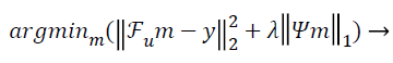
The conventional unconstrained equation used for CS in the so called Lagrangian form [10] is:
 (1)
(1)
Where  is the under-sampled Fourier operator, m is the
estimated vector, is the measured k-space data from the
scanner, λ being the regularization parameter and ψ the
sparsifying operator. Image sparsity can be enhanced either by
any sparsifying operator, or by subtracting/adding prior to
image estimation, or both [10]. The sparsifying transform used
in this paper is the finite difference transform usually referred
as Total Variation (TV) [11]. TV is the finite difference
between two consecutive rows and columns for a single line of
matrix [12].
is the under-sampled Fourier operator, m is the
estimated vector, is the measured k-space data from the
scanner, λ being the regularization parameter and ψ the
sparsifying operator. Image sparsity can be enhanced either by
any sparsifying operator, or by subtracting/adding prior to
image estimation, or both [10]. The sparsifying transform used
in this paper is the finite difference transform usually referred
as Total Variation (TV) [11]. TV is the finite difference
between two consecutive rows and columns for a single line of
matrix [12].
Trajectories
Exploring data acquisition in MRI using non-Cartesian trajectories is a viable research option as it has many advantages over the uniform-Cartesian data (Figure 1). The kspace area is well utilized, focusing essential information at the center allowing to ignore the areas on the boundary. Scan time is also significantly reduced as more phase encoding lines are skipped using non-Cartesian data [13,14].

Figure 1. Arbitrary k-space Trajectories.
The data along non-Cartesian trajectories is interpolated through Non-Uniform Fast Fourier Transform (NUFFT) using Min-Max Interpolation. The Min-Max approach provides lower approximation error than conventional interpolation error [15,16].
Gridding
The image reconstruction using non-Cartesian data is slow as compared to Cartesian data because the data is non-uniform in the k-space and we cannot apply fast Fourier transform to nonuniform data. To speed the reconstruction process gridding is used [17,18]. The main idea of gridding is to map the non- Cartesian data onto a rectilinear grid using a convolution kernel and then compensating for the convolution using an image deapodization function [9,19].
An integral part of gridding is the density compensation procedure. Unlike uniform Cartesian k-space trajectories, non- Cartesian k-space trajectories are not uniform, thus evaluating all the points as equal functions while reconstructing the data can result in major artifacts. An ideal way to perform density compensation is the post-compensation approach where we keep track of the k-space energy at each point and then divide by the particular energy after convolution [7]. But this approach is only possible if the energy is varying slowly in the data. Usually this approach doesn’t work for a majority of the k-space trajectories as it doesn’t work well with the image deapodization step [20].
The other more viable option for performing density compensation is the pre-compensation approach where density compensation is performed prior to convolution. The density of every point is measured by using a density compensation function (DCF). Many of these functions are already available and can be designed as per requirement. A simple calculation of the voronoi diagram [9] of the sample distribution is used here (this works well for most of the general trajectories). The pre-compensation technique has been adopted for the work presented in this paper.
Convolution is then performed using a pre-defined kernel function; the usual choice is the Kaiser- Bessel function [9]. The transform of the gridding kernel should be known in order to do deapodization, whichis a point-to-point multiplication of the image with the inverse of the transform kernel in order to minimize the error caused by convolution.
Methods
CS image reconstruction algorithm
Figure 2 shows all the steps of the CS reconstruction process
used in this paper. The first step is to design the k-space of the
trajectory (k) under consideration. In the second step the
Density Compensation Function (DCF) () is calculated because
we have used non-Cartesian trajectories, so the density of the
k-space samples varies throughout the data. Third step includes
the calculation of under-sampled Fourier Operator () by
taking the non-Uniform Fast Fourier Transform (NUFFT) of
the trajectory designed in the first step. In the next step undersampled,
density compensated data () is calculated by
convolving ‘w’ with ‘’. The inputs to the algorithm are the
under-sampled data (), under-sampled Fourier Operator (), Sparsifying Operator (here TV is used as the Sparsifying operator), Regularization Parameter (α or λ) and to calculate
SNR certain area for signal and noise should be declared [21].

Figure 2. Reconstruction Algorithm for Arbitrary k-space Trajectories using CS.
In this paper, the image is reconstructed using Non-Linear Conjugate Gradient Solution [10] for CS optimization problem, which uses the following equation:
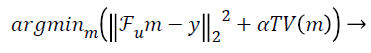 (2)
(2)
Image reconstruction algorithm using CCM and ICM
The data acquisition for CS is performed using multiple receiver coils. There are two ways to reconstruct the MR image in CS from the under-sampled data. One approach is to take the acquired under-sampled data from all the receiver coils and applying the sum-of-squares method to have a composite image, and then applying the CS algorithm to this composite image for reconstruction as shown in Figure 3a, this method is named as Collective Coil Method (CCM) in this paper. The other technique is to consider each under-sampled coil data individually for reconstruction, then applying the sum-ofsquares method to the individually reconstructed images to obtain a final result as shown in Figure 3b; this method is named as Individual Coil Method (ICM) in this paper.

Figure 3. Reconstruction Algorithm for CCM and ICM.
MR experiments
Fully sampled data is acquired using eight channel receiver coils in uniform Cartesian form. The Scan parameters used for acquiring this human head data (1.5T and 3T) are: TE=10msec, TR=500msec, FOV=20cm, Bandwidth=31.25 KHz, Slice Thickness=3mm, Flip Angle=50 degrees, Matrix Size=256x256x8. This uniform Cartesian k-space data is transformed into VD-Cartesian, Radial and Spiral trajectories and then these trajectories are under-sampled for various acceleration factors (2X, 4X, 6X, 8X, 10X).
Complex white noise (SD (σ)=0.004) is added to every data set prior to reconstruction. At different acceleration factors, the number of projections for radial trajectory vary by a factor under consideration (e.g. at 2x the total projections (256) are under-sampled by a factor of 2 etc.). The spiral trajectory used is multi-shot, the number of shots being 41 and each shot being rotated by an angle of 2π/N (where N is the number of shots).
Evaluation of reconstruction
This paper uses two quantifying parameters i.e. Artifact Power (AP) and Signal-to-Noise Ratio (SNR) to judge the quality of reconstruction.
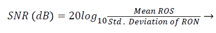
Signal-to-Noise Ratio (SNR): A Region-of-Interest for Signal (ROS) and Region-of-Interest for Noise (RON) is selected as shown in Figure 4. SNR is calculated by using the following formula [22,23]:

Figure 4. Region of Interest for SNR Calculation using Brain and Phantom data.
 (3)
(3)
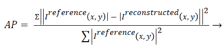
Artefact power (AP): AP is the difference between the original reference image and the reconstructed image. The concept of AP has been derived from ‘‘Normalized Sum of Square Difference Error’’. The AP in the reconstructed image is calculated on the basis of the reference image (Original Image). AP can be calculated using the following formula [22,23]:
 (4)
(4)
In the above formula, if  then AP
will be zero which tells that there is no difference between the
reference image and the reconstructed image. Similarly, if the
AP value is bigger it means there is a considerable difference
between the reconstructed image and the reference image. So
for better image the AP should be less.
then AP
will be zero which tells that there is no difference between the
reference image and the reconstructed image. Similarly, if the
AP value is bigger it means there is a considerable difference
between the reconstructed image and the reference image. So
for better image the AP should be less.
Results
Reconstruction using CCM (1.5 Tesla Head Data)
Figure 5 shows the reconstructed images, using Collective Coil Method (CCM), taken at different acceleration factors using various k-space trajectories where the acceleration factor varies vertically and the k-space trajectories are shown horizontally for the reconstructed images.

Figure 5. Reconstructed Images Using CCM.
The graph in Figure 6a shows the AP (artifact power) for VDCartesian, Radial and Spiral trajectories, whereas in Figure 6b SNR is shown for these trajectories using Collective Coil Method. The diamond (blue) represents the trend for VDCartesian, square (red) for Radial and triangle (green) for the Spiral trajectories.

Figure 6. AP and SNR Calculation for Collective Coil Method.
Reconstruction using ICM (1.5 Tesla Head Data)
Figure 7 shows the reconstructed images, using Individual Coil Method (ICM), taken at different acceleration factors using various k-space trajectories where the acceleration factor varies vertically and the k-space trajectories are shown for the reconstructed images along horizontal lines.

Figure 7. Reconstructed Images Using ICM.
The graph in Figure 8a shows the AP (artifact power) for VDCartesian, Radial and Spiral, whereas in Figure 8b the SNR is shown for these trajectories using Individual Coil Method. The diamond (blue) represents the trend for VD-Cartesian, square (red) for Radial and triangle (green) for the Spiral trajectories.

Figure 8. AP and SNR Calculation for Individual Coil Method.
Comparison CCM vs. ICM (3Tesla Head Data)
The graph in Figure 9a shows the AP (artifact power) for VDCartesian, Radial and Spiral trajectories using Collective Coil Method (CCM). The graph in Figure 9b shows the same using Individual Coil Method (ICM). The diamond (blue) represents the trend for VD-Cartesian, square (red) for Radial and triangle (green) for the Spiral trajectories.

Figure 9. AP Calculation for CCM vs ICM.
The graph in Figure 10a shows the SNR (Signal to Noise ratio) for VD-Cartesian, Radial and Spiral trajectories using Collective Coil Method (CCM). The Figure 10b shows the same using Individual Coil Method (ICM). The diamond (blue) represents the trend for VD-Cartesian, square (red) for Radial and triangle (green) for the Spiral trajectories.

Figure 10. SNR Calculation for CCM vs ICM.
Comparison CCM vs. ICM (1.5 Tesla Phantom Data)
The Figure 11 shows that the proposed method retains the high resolution features in the reconstructed image using ICM. The results have been obtained at different acceleration factors using various k-space trajectories.

Figure 11. Shows the reconstructed image of 1.5T phantom image by varying the acceleration factor for different trajectories.
Discussion
Image reconstructions are performed by implementing CS algorithm on Individual Coil Method (ICM) and Collective Coil Method (CCM) on the under-sampled VD-Cartesian, Radial and Spiral trajectories. Three different data sets (1.5T Human Brain, 3T Human Brain and 1.5T Phantom) are used to test the results for the proposed methods. The data set acquired by the 3T MR scanner provides better results in terms of AP for both methods (CCM and ICM) as compared to the data set of 1.5T scanner. In terms of SNR 1.5T human brain data provides better results as compared to 3T scanner data for ICM but for CCM the results are opposite i.e. 3T scanner data gives better output.
CS for Radial trajectory provides better results i.e. it gives smaller Artifact Power (AP) for both ICM and CCM. It performs better than variable density Cartesian. In terms of SNR, VD Cartesian trajectory outperforms both the Spiral and Radial trajectories. If we compare AP and SNR of the results generated by the two reconstruction methods, ICM provides better results in terms of AP and SNR (it gives low values for AP and higher values of SNR).
A generalization of which non-Cartesian trajectory is superior cannot be justified because certain trade-off factors are present with respect to the quantifying parameters considered but it can be safely concluded from this work that radial trajectory is a suitable choice for the CS in MRI. In terms of the method compatibility ICM shows promising results. Further work should be done in order to explore the compatibility of other non-Cartesian trajectories for CS in MRI reconstruction.
References
- Fitzgerald A, Berry E, Zinovev NN, Walker GC, Smith MA, Chamberlain JM. An introduction to medical imaging with coherent terahertz frequency radiation. Physics in Medicine and biology 2002; 47: p. R67.
- McRobbie DW, Elizabeth AM, Martin JG, Martin RP. MRI from Picture to Proton. Cambridge University Press 2006.
- Donoho DL. Compressed sensing. Information Theory, IEEE Transactions on 2006; 52: 1289-1306.
- Lustig M, David LD, Juan MS, John MP. Compressed sensing MRI. Signal Processing Magazine IEEE 2008; 25: 72-82
- Paquette M, Sylvain Merlet, Guillaume Gilbert, Rachid Deriche, Maxime Descoteaux. Comparison of sampling strategies and sparsifying transforms to improve compressed sensing diffusion spectrum imaging. Magnetic resonance in medicine 2015; 73: 401-416.
- Zijlstra F, Viergever MA, Seevinck PR. Evaluation of Variable Density and Data-Driven K-Space Undersampling for Compressed Sensing Magnetic Resonance Imaging. Investigative radiology 2016.
- Tsai CM, Nishimura DG. Reduced aliasing artifacts using variable‐density k‐space sampling trajectories. Magnetic resonance in medicine 2000; 43: 452-458.
- Li Y, Yang R, Zhang C, Zhang J, Jia S, Zhou Z. Analysis of generalized rosette trajectory for compressed sensing MRI. Medical physics 2015; 42: 5530-5544.
- Meyer CH. Fast Image Reconstruction from Non-Cartesian Data. in International society for Magnetic Resonance in Medicine 2011.
- Johnson KM, Velikina J, Wu Y, Kecskemeti S, Wieben O, Mistretta CA. Improved waveform fidelity using local HYPR reconstruction (HYPR LR). Magnetic Resonance in Medicine 2008; 59: 456-462.
- Lustig M, Donoho D, Pauly JM. Sparse MRI: The application of compressed sensing for rapid MR imaging. Magnetic resonance in medicine 2007; 58: 1182-1195.
- Block KT, Uecker M, Frahm J. Undersampled radial MRI with multiple coils. Iterative image reconstruction using a total variation constraint. Magnetic resonance in medicine 2007; 57: 1086-1098.
- Pruessmann KP, Weiger M, Scheidegger MB, Boesiger P. SENSE: sensitivity encoding for fast MRI. Magnetic resonance in medicine 1999; 42: 952-962.
- Pruessmann KP, Weiger M, Börnert P, Boesiger P. Advances in sensitivity encoding with arbitrary k‐space trajectories. Magnetic Resonance in Medicine 2001; 46: 638-651.
- Fessler JA. On NUFFT-based gridding for non-Cartesian MRI. Journal of Magnetic Resonance 2007. 188: 191-195.
- Fessler JA, Sutton BP. Nonuniform fast Fourier transforms using min-max interpolation. Signal Processing, IEEE Transactions on 2003. 51: 560-574.
- Jackson JI, Meyer CH, Nishimura DG, Macovski A. Selection of a convolution function for Fourier inversion using gridding [computerised tomography application]. Medical Imaging, IEEE Transactions on 1991; 10: 473-478.
- Beatty PJ, Nishimura DG, Pauly JM. Rapid gridding reconstruction with a minimal oversampling ratio. Medical Imaging, IEEE Transactions on 2005; 24: 799-808.
- Lustig M, Pauly JM. SPIRiT: Iterative self‐consistent parallel imaging reconstruction from arbitrary k‐space. Magnetic Resonance in Medicine 2010. 64: 457-471.
- Sedarat H, Nishimura DG. On the optimality of the gridding reconstruction algorithm. Medical Imaging, IEEE Transactions on 2000; 19: 306-317.
- Ning L, Setsompop K, Michailovich O, Makris N, Shenton ME, Westin CF, Rathi Y. A joint compressed-sensing and super-resolution approach for very high-resolution diffusion imaging. NeuroImage 2016; 125: 386-400.
- Omer H, Dickinson R. A graphical generalized implementation of SENSE reconstruction using Matlab. Concepts in Magnetic Resonance Part A 2010; 36: 178-186.
- Jim XJ, Son JB, Rane SD. PULSAR: A Matlab toolbox for parallel magnetic resonance imaging using array coils and multiple channel receivers. Concepts in Magnetic Resonance Part B: Magnetic Resonance Engineering 2007. 31: 24-36.