Research Article - Biomedical Research (2017) Artificial Intelligent Techniques for Bio Medical Signal Processing: Edition-I
Fault tolerant topology control with mobility prediction in MANETs for clinical care data transmission
D Manohari1*, GS Anandha Mala2 and KM Anand Kumar21St. Joseph’s College of Engineering, Chennai, India
2Easwari Engineering College, Chennai, India
Accepted on January, 09, 2017
Abstract
One of the main issues with MANET is Topology control arising due to its dynamic nature. Efficient control of topology in MANET is possible only when mobility prediction is done to avoid any kind of interruption in the communication. In this work, neural network based mobility prediction model for topology control is proposed. In this prediction model a highly scalable and accurate multi-layer architecture is exploited to perform N-step prediction to forecast the future location of the mobile nodes. The optimal path is then selected based on the minimum interference, transmission power values of nodes and the path availability using Ant Colony Optimization (ACO) technique. Clinical care data is collected during the course of ongoing patient care. The proposed method provides uninterrupted communication for transferring clinical care data like details about rehabilitation hospitals for patients. The simulation results obtained prove that the proposed technique is successful in reducing the packet drop, transmission delay and improves the packet delivery ratio as well as residual energy.
Keywords
Topology control, Ant colony optimization, MANET.
Introduction
Mobile ad-hoc network (MANET)
Mobile Ad-hoc Network (MANET) consists of a set of selforganized mobile nodes that are associated with low bandwidth wireless links. Each node has its own area of control called “cell”. In MANETs, there are no fixed infrastructures and the nodes are free to move due to which the network topology may change rapidly over time. This results in the nodes preparing their own acceptable infrastructures [1-3]. Clinical data is a essential resource for most health and medical research. The different types of Clinical data include Electronic health records, administrative data ,Claims data , Patient / Disease registries, Health surveys and Clinical trials data.
Mobility prediction in mobile ad-hoc networks
Mobility Prediction of a node is referred to as the capacity to evaluate a future position given past positions [4]. It is used in location supported routing and mobility aware topology control protocols [5]. These protocols predict the future location of each node easily and forecast parameters such as future distance between two neighboring nodes.
The major issue of mobility prediction is the inaccuracy in the future distances forecaster. The effectiveness of this forecaster may vary due to the presence of unusual mobility models, sampling rates and dissimilar speed ranges [5]. Unpredictable changes in the user’s behavior are also a major issue in mobility prediction. Due to dynamic topology and non-regular rations in such functions, node mobility forecast based on the movement history is not feasible and effective. For most of the MANET applications, group and node velocities are time variant which affects the accuracy of location predictor [6].
Issues in topology control in mobile ad-hoc networks
Topology control is mandatory due to the continuous change in the primary topology of the network. A centralized approach can achieve strong connectivity but has many scalability issues. In contrast, a distributed approach is scalable but lacks the strong connectivity guarantees and consumes a large amount of power [7].
Literature Review
Aiyud et al. [8] discussed Group Mobility Prediction in Mobile Ad-hoc Network. The authors applied a data mining technique to forecast behavioral group patterns consequential from user movement’s data in a mobile computing system. The proposed algorithm is based on mining the mobility patterns of users in each group, forming mobility rules from these patterns and finally predicting a mobile user’s group movement by the declared mobility rules. The performance metric discussed is latency which is reduced. The proposed algorithm may not match or may be only a miniscule match to any of the mobility rules to the present trajectory of a mobile user. So, no prediction can be consummate in various cases when the exploitation gets very high.
Hakki Bagci et al. [9] have discussed about fault tolerant topology control in ad-hoc networks. This work proposed a disjoint path vector algorithm where k- disjoint paths between source and destination. At worst case there will be single link between the nodes atter all link failures. Yassir et al. [10] proposed a user profile-based location prediction based on the neural networks concept. Elman networks were used and a probability of 85% was achieved to identify the right location area. Asha et al. [11] proposed Network Connectivity based Topology Control (NCTC) to establish the balance between interference and energy to enhance the network lifetime of networks. In this scheme, first, interference was reduced and further, the efficient topology control based on energy constraint was proposed to extend the network lifetime of networks. Performance metrics like network lifetime, packet delivery ratio, less overhead and end to end delay has been analyzed. During Link Weight Information Exchange, each node performed the weight calculations for all links. Hence, this approach required more computation time and stricter preconditions which may cause computational overhead.
Distance Vector (DV) unicast protocol enhanced with mobility prediction offers packet delivery ratios of 0.9 (i.e., 10% of packet loss) for speeds up to 70 km/h. Also, the On-Demand Multicast Routing Protocol (ODMRP) [12] with mobility prediction performs better than its counterpart without prediction and offers packet delivery ratio of 0.9 (i.e., 10% of packet loss) for speeds up to 70 km/h [13].
Proposed Solution
Literature survey disclosed the fact that a scheme with a capability to provide fault tolerant topology control and mobility prediction together is required. To accomplish this, the link availability estimation technique analyzed by Teotia and Garg [14] was merged with neural network based prediction model evaluated by Kannche and Kamoun in their work [9]. The following sections discuss the details of the proposed work.
Overview
In earlier work [15], topology control in MANETs had been clutched through swarm intelligence. Each node constructs its neighbor set by sending a neighbor discovery message to its neighbors. The fault tolerant path is identified by estimating minimum transmission consumption and minimum interference path. To augment the previous work, mobility prediction with topology control was performed to find the most reliable path for unremitting communication. Optimal path is selected based on the interference, transmission power values of nodes and path availability. The minimum interference and transmission power values of nodes are determined using Ant Colony Optimization and path availability by neural network mobility prediction method.
The different phases of the proposed model are explained as follows. The first one is the use of swarm intelligence to find the transmission power and interference of neighbor nodes using ant agents. Subsequently, the phase deploys Neural Network Based Prediction model [9] was used in which the recurrent multi-layer neural network with three layers was utilized to predict the mobility of neighbor nodes. Finally, based on the prediction, path availability and the time period of its existence were estimated [14]. The following section explains multilayer neural network architecture for mobility prediction.
Multi- layer neural network architecture
Three main layers that are arranged in a feed forward fashion are used for mobility prediction as shown in Figure 1.

Figure 1: Multilayer based mobility prediction architecture.
Input layer: The main function of network input layer in Nstep prediction is accepting time series observations along with estimated input coming from the previous network. In each prediction step k where k ≠ N, the network output p̂(t+k) is stored in the input layer so that it is able to estimate the value p̂(t+k). This is done based on feedback connection between output neuron and a neuron in the input layer.
Hidden layer: The second layer is called as hidden layer. The main function of this layer is to store the characteristics of the known patterns to increase the freedom of degree in the problem resolution to improve the generalization ability of the network.
Output layer: This layer receives the different prediction values from the input layer and after evaluating the values it sends the feedback to input layer.
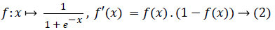
Notations: The different notational conventions used for neural architecture are the Ne, Nc and Np which denotes the number of neurons in input, hidden and output layers respectively. The values that have been assigned for Ne where e= {1……….Ne}, Nc c= {1………….. Nc} and Np p=1. In this bias terms are obtained by adding a bias neuron in both input and hidden layer whose input have constant value which is equal to 1. Iv represents the weighted sum of the input which is calculated by neuron v of either hidden or output layer. Iv is computed at each neuron becomes argument of a sigmoid activation function and stays in the neuron itself. Ov is the value returned by the activation function of neuron v as given in the equation (1).
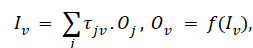 → (1)
→ (1)
The N-step multilayer mobility prediction algorithm: The proposed prediction algorithm can be described briefly as follows.
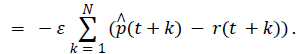
Step 1: In the prediction step k, a real observation r(t+k) is forecasted as p̂(t+k) which corresponds to network output. The quantity Jk is used in the eq (3) in order tp denotes the square error function in prediction step k.
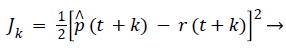 (3)
(3)
The total error function in prediction step N is given as the summation of error functions Jk that corresponds to prediction step k.
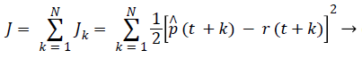 (4)
(4)
Step 2: The network is then made qualified using Back Propagation through Time (BPTT) algorithm by minimizing the error function J.
Step 3: The weights are then modified at the time (t+N) which corresponds to the Nth prediction step with the help of function error J.
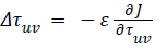
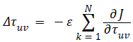
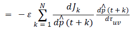 → (5)
→ (5)
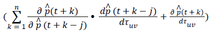
Here, n represents number of forecasted inputs from the input
layer since the network output is re injected in the input layer.The quantities and
and  is given by:
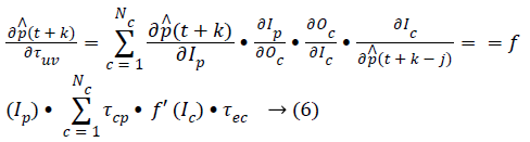 Here, the weight ωec represents the weight of the link
connecting the neuron e in the input layer whose input is s (t +
k- j) and a neuron c in the hidden layer.
Here, the weight ωec represents the weight of the link
connecting the neuron e in the input layer whose input is s (t +
k- j) and a neuron c in the hidden layer.
 (7)
(7)
The Random Way Point (RWP) Mobility model is used to construct the location time series. In this model, a mobile node starts from its current position and chooses randomly a destination position in its mobility region. Then, it moves straight towards this destination with a constant speed, chosen randomly in various intervals of speed. When it reaches the destination, it remains stable for a period of time and then restarts the same movement process.
Link availability prediction
The different metrics used in this work can be explained briefly in the following sections.
Estimation of metrics: PT and L(PT). This section describes two metrics which are used to find the link expiration time and subsequently path expiration time. The time period (PT) during which link exists between nodes is predicted by assuming that both nodes move with same speed and direction. Then, the probability L(PT) of link availability during the time period t0 to PT is estimated by considering changes in the nodes’ movements as given in equation (8).
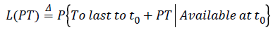 → (8)
→ (8)
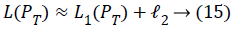
Equation (8) implies probability that the existence of link availability throughout the time interval t0 and t0+PT. L(PT) comprises of two components namely L1(PT) which gives the probability of the existence of link availability between two nodes with their velocity remains constant and L2 (PT) for other cases.
L(PT) = L1(PT) + L2(PT) → (9)
Calculation of L1 (PT): Assuming the random length interval (epoch) in which each node moves in a constant direction at a constant speed, then the expected value of time is
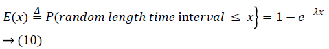
Since the movement of nodes follow an exponential distribution and are independent of each other, L1(PT) can be calculated as follows.
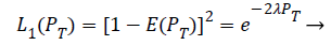 (11)
(11)
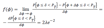
Calculation of L2(PT): Let δ be the random time interval during which there is a change in movement of the nodes and Φ be the random interval where the nodes keep their movements unchanged. Thus, the change in movement of either one node or both will occur only after t0 + Φ. To calculate L2(PT) the probability should be considered as follows

The probability for Φ is given by
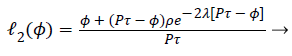 (13)
(13)
p - is the probability for the two nodes to move to closer each other after changing their movements. Since there is equal probability for the nodes to move to closer each other or far apart, probability value for p is 0.5. φ ≥ 0 - is the adjustment to link availability depends on factors such as node density and radio coverage of the node. Consider the first change in the movement of the nodes occur at t0 + Φ. From t0 + Φ to t0. + PT, total time (Tt) that a link will be continuously available can be formulated as
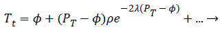 (14)
(14)
For the movement changes in the remaining time period the above calculation has to be repeated to calculate the ‘…’ in eq. (14).
The average value  is used to estimate L2 (PT).
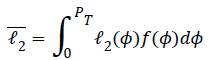
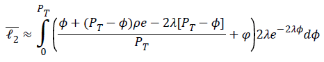
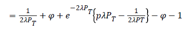
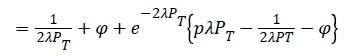
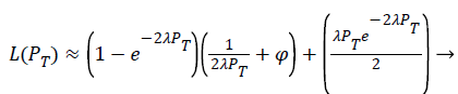 (16)
(16)
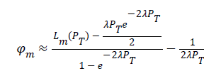
Calculation of Φ: In order to make the proposed estimation algorithm adaptable to environmental changes, the value of φ is measured as follows. After the prediction of link availability PT using equation (16) the real observed value PR during which the link is really available is measured. This will be repeated a number of times to record PR value and the number of occurrences (nr) that have the same PR value. Measured PT value Lm(PT) is calculated.
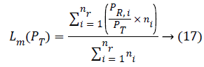
Substituting eq. (17) in eq. (16) φm measured value is
Optimal path selection
Neighbor set (NS) construction: Initially after all nodes are deployed in the network, each node broadcast NEI_DIS (Neighbor Discovery) message to discover its neighbors. Nodes that receive NEI_DIS message, sends back the ACK message.
The ACK message holds node id, sequence number and hop count. Each node waits for a time twait to receive ACK message from all possible neighbors. After the expiration of twait, it constructs the Neighbor Set (NS) by retrieving the information from ACK messages. The NS table format is given below in Table 1.
| Node ID | Seq. No | HopCount | ChosenTrans Power | Interference No | Link Availability Duration |
Table 1. NS table format.
In the above table, CH Trans Power will be updated by ant agent and interference number by IN_NUM packets. Consider network is designed as a communication graph G (V, E). Where, V represents nodes and E denotes the link. Let ni, nj, nk … nn-1 be the set of mobile nodes. During transmission of data from ni to nj, node ni may interfere the nodes that are nearer to ni and nj. Unidirectional interference set (UDI) contains the set of nodes that are interfered by ni’s transmission to nj. UDI (ni, nj) can be estimated by,

Where, nk is a neighbor node and dis (ni, nj) be the euclidean distance between ni, nj. Optimal path from the source s to destination d can be obtained by relating interference, transmission power values of nodes and path availability duration. Optimal path selection process is portrayed in algorithm 1
Algorithm 1
Step 1: Each node calculates its transmission power and its interference number which are described in previous work [15].
Step 2: Link availability duration (Pa) is estimated using Nstep neural network based prediction.
Step 3: Forward and backward ants are employed to collect CH Trans Power of nodes.
Step 4: Transmission power (TP) of each path is determined by aggregating the CH Trans Power values of all nodes in that path.
TP (Pn) = CH Trans Poweri
Where, i= 1, 2, 3… n=1, 2, 3…
Step 5: The interference numbers of the node are accumulated by sending IN_NUM message packets.
Step 6: Interference number (IPn) of each path is calculated. The values of TP, IPn and path availability durations are stored in NS table.
Step 7: Select the path that satisfies Popt=min{TP (Pn)} and min {IPn}, and Max {Pa}.
Where the minimum transmission power and interference number is found by using Ant Colony Optimization (ACO).
Step 8: The path (Popt) is selected for data transmission from the source to the destination.
In Figure 2, nodes 2, 3, 4… 14 are deployed randomly. P1, P2, P3 and P4 are paths that connect source and destination. S- 6- 8- D is the optimal path since it has minimum transmission power and interference and maximum path availability duration.

Figure 2: Optimal path selection.
Simulation Results
Simulation model and parameters
The Network Simulator (NS2) [16] is used to simulate the proposed architecture. The simulation has been performed for different scenarios, one by keeping transmission range constant and the other by varying the transmission range of the mobile nodes; 50 to 100 mobile nodes move according to RWP mobility model in 1000 meter × 1000 meter region for 100 seconds of simulation time with the same transmission range of 250 meters and the simulated traffic is Constant Bit Rate (CBR). Data for transmission is taken from dataset that contains details about rehabilitation hospitals which are equipped with inpatient wards for evaluation and restoration of function to patients who have lost function due to acute or chronic pain, musculoskeletal problems, stroke, or catastrophic events resulting [17].
Two location time series x(t-i) {i= 0.. 20} and y(t-i) {i= 0..20} have been obtained. From the observation, 5 sets of data were taken and prediction was done for the same. The first 50 pair of co-ordinates was used for training and the rest for generalization. The NN based predictor was tested on these two location time series to predict the movement of mobile nodes. The parameters Ne and Nc were fixed respectively at 10 and 5. The simulation settings and parameters are summarized in table.
| No. of Nodes | 50, 100,150,and 200 |
| Area Size | 1000 × 1000 |
| MAC | IEEE 802.11 |
| Transmission Range | 250m (scenario 1) and 250m, 450 m(scenario 2) |
| Simulation Time | 100 sec |
| Routing Protocol | SWARM |
| Initial Energy | 15.3 J |
| Receiving Power | 0.395 |
| TransmissionPower | 0.660 |
| Bit Rate | 200kb |
| Speed | 5,10,15,20 and 25m/s |
Table 2. Simulation parameters.
Performance metrics
The proposed swarm based topology control for fault tolerance with neural network based mobility prediction (SwarmFTCP) is compared with the Local Minimum Interference Biconnected Communication Networks LMIBCN method [11]. In LMIBCN fault tolerance was implemented in terms of interference alone whereas the proposed method has identified a path between a source and destination with minimum interference, minimum power consumption and highly stable path. The performance is evaluated mainly primarily according to the following metrics.
• Packet delivery ratio: It is the ratio between the number of packets received and the number of packets sent.
• Packet drop: It refers to the average number of packets dropped during the transmission.
• Energy consumption: It is the amount of energy remains in the nodes after the data packet transmission.
• End-to-end delay: It refers to the time taken for a packet to be transmitted across a network from source to destination.
Results
Based on speed with constant transmission range: In this experiment, the speed of the mobile nodes is varied as 5,10,15,20 and 25 m/s for which the number of nodes is varied from 20 to 60 nodes. The performance of the techniques is as illustrated in the Figures 3-5.

Figure 3: Speed vs. Delay.

Figure 4: Speed vs. Delivery ratio.

Figure 5: Speed vs. Residual energy.
From the above results, it is found that the proposed swarmFTCP outperformed LMIBCN. The observation of delay incurred during the transmission of packet from source to destination in Figure 3 revealed the fact that at lower speeds performance of both techniques is almost the same. When speed is gradually increased in steps of 5 m/s end-to-end-delay also increased and attained a maximum at 15 m/s. Subsequently there is a decrease in end-to-end-delay in both techniques due to the mobility prediction in swarmFTCP and interference calculation in LMIBCN. Delay incurred in swarmFTCP is 13% less than that of LMIBCN. Figures 4 and 5 shows the delivery ratio and residual energy of SwarmFTCP and LMIBCN techniques for different mobile speed scenario respectively. The packet delivery rate is reduced with increasing mobility due to increased link breaks. When the speed increases, the links between two nodes often break,followed by more packet losses and thus, fewer packets are delivered to the destination. SwarmFTCP provides better performance than LMIBCN due to its prediction capability and packet delivery ratio is 43% greater than that of LMIBCN. There occurred an increase in route failures as speed is increased and hence the possibility of alternate routing will be more. Therefore, residual energy of LMIBCN is 20% less than that of swarm FTCP.
Based on number of nodes with constant transmission range: Next the performance of swarmFTCP and LMIBCN was analyzed by varying the number of mobile nodes from 50 to 200. Figure 6 shows the end-to-end delay of SwarmFTCP and LMIBCN techniques for different number of mobile nodes. There is an increase in delay detected because of increase in number of nodes which increases total traffic load and thus, the network becomes congested. This leads to more packets in queues for a long time which causes the delay to increase. However, swarmFTCP outperforms LMIBCN in reducing the end to end delay of range 9 – 10%. The delivery ratio of SwarmFTCP is 52% more than LMIBCN and residual energy of SwarmFTCP is 22% lesser than that of LMIBCN. This is shown in Figures 7 and 8. Compared to LMIBCN the delivery ratio of swarmFTCP is a bit high, which is due to its ability to select a set of stable and least congested routes thus having the lowest amount of packet loss and very few route failures.

Figure 6: Nodes vs. Delay.

Figure 7: Nodes vs. Delivery ratio.

Figure 8: Nodes vs. Energy.
Based on transmission range: In this experiment, the transmission range is varied from 250 m to 450 m. Since routing through multiple hops will occur during low transmission power, there is an increase in end-to-end delay. But beyond the 250 m transmission range, the end to end delay was very much reduced to a very lower level. When the transmission range is highest, routing overhead is minimum and at lowest transmission range routing overhead in maximum. LMIBCN suffers a lot in larger transmission range as more interference is rooted. It has been found from Figures 9-11 that there is high end-to-end delay, less packet delivery ratio and less residual energy for LMIBCN. SwarmFTCP provides better performance in different transmission ranges as it incorporates mobility prediction for finding a stable path which less power consumption and reduced interference. SwarmFTCP has 14% less delay, 36% greater packet delivery ratio and 22% higher residual energy than that of LMIBCN.

Figure 9: Range vs. Delay.

Figure 10: Range vs. Delivery ratio.

Figure 11: Range vs. Energy.
Conclusion
In this work, neural network based prediction model for topology control in MANET that consists of three layers to perform N- step prediction of object’s location is proposed. This model is highly scalable and accurate. The proposed method provides a technique not only for mobility prediction but provides both a most reliable and a stable path for the communication about the details of rehabilitation hospitals to the patients without any interruption in the network. Based on the interference, transmission power values of nodes and path availability, the optimal path is selected for data transmission using Ant Colony Optimization. Through simulation, it is proved that the proposed technique reduces the packet drop, delay and improves the packet delivery ratio and residual energy. Future work may be done by increasing the step value N in prediction of mobile nodes’ location to improve the stability of path.
References
- Xing Z, Gruenwald L. Issues in Designing Concurrency Control Techniques for Mobile Ad-hoc Network Databases. Technical Report, School of Computer Science, University of Oklahoma, July 2007.
- Mukilan P, Wahi A. NMDRA: Efficient Energy and Node Mobility based Data Replication Algorithm for MANET. IJCSI Int J Comput Sci Issues 2012; 9: 357-364.
- Moon A, Cho H. Energy Efficient Replication Extended Database State Machine in Mobile Ad-Hoc Network. IADIS International Conference on Applied Computing, 2004.
- Nagaraj U, Bharane A, Chaudhari B, Naidu A. Mobility Prediction and Routing in Vehicular Ad hoc Network. Int J Eng Res Appl (IJERA) 2012; 2: 1514-1518.
- Mousavi SM, Rabiee HR, Moshref M, Dabirmoghaddam A. Model Based Adaptive Mobility Prediction in Mobile Ad-Hoc Networks. IEEE Wireless Commun Network Mobile Comput 2007; 2007: 1713-1716.
- Gavalas D, Konstantopoulos C, Mamalis B, Grammatiantziou B. Mobility Prediction in Mobile Ad Hoc Networks. Next Generation Mobile Networks and Ubiquitous Computing. In: Encyclopedia of Next Generation Networks and Ubiquitous Computing, Ed: Samuel Pierre, IGI Global, Hershey, USA, 2011.
- Ashwini V, Patil S. Topology Control in Wireless Sensor Network: An Overview. Int J Comput Appl 2014; 92: 13-18.
- Romsaiyud W, Premchaiswadi W, Premchaiswadi N. An Autonomous Group Mobility Prediction Model for Simulation of Mobile Ad-hoc through Wireless Network. J Wireless Network Commun 2012; 2: 126-135.
- Bagci H, Korpeoglu I, Yazıcı A. A Distributed Fault-Tolerant Topology Control Algorithm for Heterogeneous Wireless Sensor Networks. IEEE Transact Parallel Distributed Syst 2015; 26: 914-923.
- Yassir A, Abdel-asir G, Roy P. Mobile Ad-hoc Networks Location Prediction by using Artificial Neural Networks: Considerations and Future Directions. Int J Computer Technol Appl 2013; 4: 120-125.
- Asha TS, Muniraj NJ. Network Connectivity based Topology Control for Mobile Ad Hoc Networks. Int J Comput Appl 2012.
- Sung-ju L, Su W, Gerla M. Wireless Ad Hoc Multicast Routing with Mobility prediction. J Mobile Networks Appl 2001; 6: 351-360.
- Chellappa-Doss R, Jennings A, Shenoy N. A review on Current work in mobility prediction for wireless networks. Proceedings of the 3rd Asian International Mobile Computing Conference, 2004.
- Teotia S, Garg S. A Characteristic Study of Mobility Models Prediction Methods for MANETs. Int J Eng Adv Technol (IJEAT) 2012.
- Manohari D, Anandha Mala GS. Swarm Based Topology Control for Fault Tolerance in MANET. Int Rev Comput Software (IRECOS), 2013.
- http: //www.isi.edu/nam/ns
- https://www.healthdata.gov/search/type/dataset