Research Article - Biomedical Research (2017) Volume 28, Issue 17
Effective ECG beat classification using higher order statistic features and genetic feature selection
Yasin Kaya1*, Hüseyin Pehlivan1 and Mehmet Emin Tenekeci2
1Department of Computer Engineering, Karadeniz Technical University, Trabzon, Turkey
2Department of Computer Engineering, Harran University, Şanlıurfa, Turkey
- *Corresponding Author:
- Yasin Kaya
Department of Computer Engineering
Karadeniz Technical University
Trabzon, Turkey
Accepted on August 16, 2017
Abstract
One of the most significant indicators of heart disease is arrhythmia. Detection of arrhythmias plays an important role in the prediction of possible cardiac failure. This study aimed to find an efficient machine-learning method for arrhythmia classification by applying feature extraction, dimension reduction and classification techniques. The arrhythmia classification model evaluation was achieved in a three-step process. In the first step, the statistical and temporal features for one heartbeat were calculated. In the second, Genetic Algorithms (GAs), Independent Component Analysis (ICA) and Principal Component Analysis (PCA) were used for feature size reduction. In the last step, Decision Tree (DT), Support Vector Machine (SVM), Neural Network (NN) and K-Nearest Neighbour (K-NN) classification methods were employed for classification. The proposed classification scheme categorizes nine types of Electrocardiogram (ECG) beats. The experimental results were compared in terms of sensitivity, specificity and accuracy performance metrics. The K-NN classifier attained classification accuracy rates of 98.86% and 99.11% using PCA and ICA features. The SVM classifier achieved its best classification accuracy rate of 98.92% using statistical and temporal features. The K-NN classifier feeding genetic algorithm features achieved the highest classification accuracy, sensitivity, and specificity rates of 99.30%, 98.84% and 98.40%, respectively. The results demonstrated that the proposed approach had the ability to distinguish ECG arrhythmias with acceptable classification accuracy. Furthermore, the proposed approach can be used to support the cardiologist in the detection of cardiac disorders.
Keywords
Electrocardiogram (ECG), Arrhythmia, Classification, K-nearest neighbour (K-NN), Neural network, Support vector machine (SVM), Genetic algorithms, Principal component analysis (PCA), Independent component analysis (ICA).
Introduction
Electrocardiogram (ECG) signals show electrical activity of the heart. The signals are used for early diagnosis of heart abnormalities and record changes in the heart [1,2]. Heart arrhythmias occur with deviation from the normal physiological behaviour of the heart. They are usually associated with abnormal pumping function and are caused by any interruption in the regularity, rate, or conduction of the electrical impulse of heart. Arrhythmias decrease the quality of life for the patient and can even cause sudden death [1,3]. The automatic separation of ECG heartbeats into sub-categories can be used in computer-aided diagnosis. It reduces the time spent by cardiologists on the analysis of these records. An effective ECG heart beat classification generally includes three important modules: feature extraction (calculation), feature selection (dimension reduction) and construct classifier scheme. Feature extraction and reduction are two important steps as they frequently affect the classification performance of any heartbeat classification system. Consequently, the main tasks of arrhythmia classification problems are the extraction of adequate features and the reduction of their sizes for classifiers in order to accomplish optimal classification results [4].
Studies indicate that various feature extraction, dimensionality reduction and classification methods have successfully implemented arrhythmia classification and other pattern recognition problems. The feature extraction methods include vector quantization, the Lyapunov exponent, Wavelet Transform (WT), spectral correlation, statistical methods, and the Fourier transform [3-13]. The PCA, GA, ICA and Self- Organizing Map (SOM) methods were used for dimensionality reduction [1,3,4,9,10,14-19]. Researchers have extensively used NN, SVM, DT, logistic regression, modified artificial bee colony algorithm, classification and regression tree, Neuro-fuzzy system, and K-NN classification methods [3,4,8-11,13,17,20-31].
Das et al. proposed an ECG classification method using the Stockwell transform (S-transform) in their study. The S-transform was used for the calculation of morphological features. NN and SVM classification methods were employed as classifiers [20]. Thomas et al. used features calculated with WT for ECG classification. A multi-layered NN classifier was used in their study. The performance of the proposed feature set was compared with the features extracted by Discrete Wavelet Transform (DWT) sub-band decomposition in the QRS complex. One normal and four abnormal beats were classified in the study [11]. Dilmac et al. used a modified bee colony algorithm to classify ECG beats. In their study, the morphological attributes of the QRS complex and the time interval between heartbeats were used as features. Three beat types taken from the MIT-BIH arrhythmia database were classified. The obtained results were compared with several classifiers used in the literature [29]. Khalaf et al. proposed a model for the classification of ECG arrhythmias. Spectral correlation and PCA were used for feature extraction and SVM was used as a classifier in the study. For the experimental results, they used five beat types [3]. In another study, the authors used hermit transformation coefficients and R-R time intervals as features [21]. Chazal et al. used ECG morphological information and R-R time intervals as features in their work [32]. Liu et al. proposed a dictionary learning algorithm that employed k-medoids clustering optimized by k-means++. They used a vector quantization algorithm for feature extraction. In the study, 1200 beats of eight types from different databases in the MIT-BIH were taken for the experimental results [5]. Nazarahari et al. used wavelet functions to calculate features for the classification of ECG beats. They used a multi-layered NN as a classifier and PCA for dimension reduction. In their study, one normal and five abnormal beat types were classified and the results compared [9]. In another study, the authors proposed a Continuous Wavelet Transform (CWT) based approach for ECG arrhythmia classification. They used a GA to develop a new WT-based classifier [10]. Sumathi et al. proposed a hybrid method using ANFIS which analyzed the ECG signal on the basis of symlet wavelets. They extracted the parameters associated with dangerous heart disease and used these parameters in ANFIS to classify five types of ECG beats [8].
Melgani et al. focused on a SVM-based approach to automatic diagnosis of ECG beats in their study. In addition, the Particle Swarm Optimization (PSO) method was used and the ability of the SVM algorithm to generalize was advanced [25]. Güler et al. used a combined NN to classify ECG beats. The ECG signal was decomposed using WT for the time-frequency representation in the study. They calculated the statistical values representing the distribution and classified four beat types [7]. Engin applied neuro-fuzzy networks for ECG beat classification. He used higher-order cumulants, autoregressive model coefficients and WT variances as features for arrhythmia recognition. Four types of beats were used for the experimental results [23]. Osowski et al. focused on a fuzzy-hybrid NN for ECG arrhythmia classification. They used Gustafsol-Kessel algorithms for self-organizing the NN [33].
In a more recent work, Premature Ventricular Contraction (PVC) was classified through visual features extracted from a considerable set of ECG signals. The authors analyzed time series features with respect to the classification performance of PVC arrhythmia. The performance evaluation was also conducted on the effects of some dimension reduction methods [1]. All these studies were based on ECG signals provided by the MIT-BIH arrhythmia database for their experimental tests [34].
A whole heartbeat was used for feature extraction in the studies related to arrhythmia classification. However, a heartbeat contains information about different characteristic (P waves, the QRS complex, T and U waves) [4,35]. In this study, one beat signal was divided into four equal sections and new statistics-based features were calculated to reveal this information. These new features were used in the classification approach. In order to test the proposed approach, nine types of ECG beats taken from the MIT-BIH arrhythmia database were used [34]. Test results show that the proposed approach attained classification accuracy rates of 98.86% using a K-NN classifier. Subsequently, different dimension reduction algorithms were used in order to determine the most effective features, and the classification performance was increased to 99.30%.
Materials and Methods
Figure 1 demonstrates a block diagram of the heartbeat classification scheme proposed in this study. The noise and fluctuations were removed from the signal in the pre-processing step.

Figure 1. Block diagram of the proposed heartbeat classification scheme.
The signal was parsed to beats in the beat-parsing step. Statistical and time interval features of the signal (whole beat and four equal sections) were calculated in the feature-extraction step. Three different dimension reduction algorithms were performed for the calculated features. The PCA and ICA were implemented to decrease the size of the feature vector. The GA was used to select the best features to represent all the features. In this step, parameter optimization was performed in order to calculate the parameters achieving better results. In the classification step, the DT, SVM, K-NN, and NN algorithms were employed, their results were compared, and the classification scheme achieving the best results was determined.
ECG database
The study employed a data set of 48 signals obtained from the MIT-BIH arrhythmia database [34,36]. Each signal in the set, which was 30 min in duration and included two important leads (i.e., Lead II and a modified one), was sampled at 360 Hz. 23 files of signals were randomly selected, which were supposed to represent routine clinical records. The remaining 25 files were chosen associated with rare complex junctional, supraventricular and ventricular arrhythmias. The database was annotated with beat label and timing information. In particular, the labels were used to determine the position of the beats contained by the signal files. A random selection procedure was used in this work. This included a total of 6318 samples for nine different types of ECG beats in the MIT-BIH arrhythmia database. These typical ECG beats are left bundle branch block (L), premature ventricular contraction (V), right bundle branch block (R), paced beat (P or /), fusion of paced and normal beat (f), fusion of ventricular and normal beat (F), ventricular escape beat (E), aberrated atrial premature beat (a), and normal beat (N). When there were more than 1000 samples for one beat type in database, 1000 samples were selected, otherwise all samples were selected.
Pre-processing
The oscillations in the ECG signals lead to an undesirable effect on the features calculated for them, decreasing the performance of the signal processing algorithms [2,37]. A particular type of ECG signals recorded from the people can exhibit notable differences. Noises were generally found in the signals recorded during the patient’s natural daily behaviour such as breathing, coughing, and bending. The normalization and pre-processing operations performed on the signal remove the noise and decrease its effects on the calculated features.
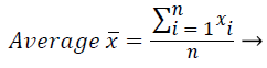
In this work, setting the mean of the ECG signal to 0, the calculation load of the mathematical operation is reduced. The zero-mean signal y (t), t=1, 2, … , L was calculated by equation (1): y (t)=x (t)-͞x------(1)
Where ͞x corresponds to the arithmetic mean of the raw ECG of x (t), t=1, 2, … , L and L is the signal length.
In the next step, using a cascade filter, frequency components below 0.5 and 2 Hz are removed from the signal of y (t) and thus the baseline wander is eliminated. The baseline wander usually has the frequency components of below 0.5 Hz. However, given some situations such as a stress test, the components can have a higher frequency [1]. Therefore, the upper bound of the frequency is limited to 2 Hz. Figure 2 shows (a) The raw signal; (b) Cascade filter result; (c) Filtered signal of the first 14 seconds of signal file 203. In Figure 2 (c), the baseline wander was subtracted from the signal to obtain a smoother baseline.

Figure 2. (a) Raw signal, (b) cascade filter result and (c) filtered signal.
Beat parsing
Every beat in the ECG must be separated and constructed in a single beat format before feature extraction. In accordance with to the location of the QRS complex, the ECG signal is used to extract window length of 200 points for each beat [1]. These points are established on the left and right sides of the R point, respectively with 99 and 100 ones, and the remaining one point is done on the R point itself. With the help of the annotation files of the MIT-BIH database, the location of the R point was gathered for the related beat.
Feature extraction
Subspace domain features, morphological features, and statistics-based features are usually preferred as features for arrhythmia classification [8-11,20,29,31].
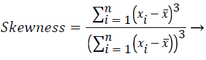
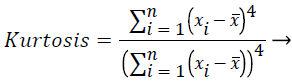
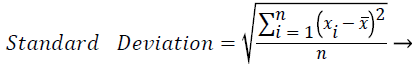
In this study, amplitude values of 200 sample points gathered in the beat-parsing step were used to calculate the statistical features. The skewness, kurtosis, distribution range, interquartile range, standard deviation, and average statistical features were calculated for these values.
These features were calculated over the entire beat and each of the four equal-width regions are shown in Figure 3. Dashed lines in the figure indicate the border of the region.

Figure 3. Calculating features from one beat and its sections.
The first region border ends approximately at the top of the P wave, the second region border ends at the R point, and the third region border ends approximately at the T wave.
These features were calculated as in equations (2-7):
 (2)
(2)
 (3)
(3)
Range=Maximum (xi)-Minimum (xi), i=1…n (4)
Interquartile range=Q3-Q1 (5)
 (6)
(6)
 (7)
(7)
Where xi is the ith sample value, n is the sample count, and ͞x is the mean of the examples.
The distribution range is calculated as the difference between the largest and smallest of these values. The interquartile range is a statistical measure of dispersion and is equal to the difference between the lower (Q1) and upper (Q3) quartiles. The quartiles split a rank-ordered data set into four equal fragments. The values that split each fragment are called the first, second, and third quartiles and they are represented by Q1, Q2 and Q3, respectively. The standard deviation is a measure of the statistical distribution of the data and equal to the square root of the variance. Table 1 shows the calculated statistical features. In this work, the time interval for the active beat between the previous and next beat was used as a feature. For this purpose, the R-R previous (RRP) and R-R after (RRA) values were calculated (Table 2). After this addition, the size of the feature vector was identified as 32.
| Statistical features | ||||||
|---|---|---|---|---|---|---|
| Feature | Skewness | Kurtosis | Range | Interquartile range | Standard deviation | Mean |
| Whole beat | SKEW0 | KURT0 | RANG0 | IQR0 | STD0 | MEA0 |
| Section 1 | SKEW1 | KURT1 | RANG1 | IQR1 | STD1 | MEA1 |
| Section 2 | SKEW2 | KURT2 | RANG2 | IQR2 | STD2 | MEA2 |
| Section 3 | SKEW3 | KURT3 | RANG3 | IQR3 | STD3 | MEA3 |
| Section 4 | SKEW4 | KURT4 | RANG4 | IQR4 | STD4 | MEA4 |
Table 1. Calculated statistical features.
| Time-related features | ||
|---|---|---|
| Feature | R-R Previous | R-R After |
| Whole beat | RRP | RRA |
Table 2. Calculated time-related features.
Performance measures
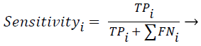
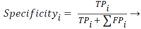
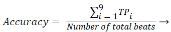
Sensitivity, specificity and accuracy performance metrics were used to compare classification results. Although the accuracy metric was a single value in the multi-class classification, sensitivity and specificity metrics were not single values and were calculated individually by each class. Equations (8-10) show the performance measures for multi-class classification.
 (8)
(8)
 (9)
(9)
 (10)
(10)
Where the subscript i represents the class label, TP symbolizes the true positive, FP symbolizes the false positive, and FN symbolizes the false negative for each class.
Results
The performance of heartbeat classification systems depended on several important factors including classification methods applied, the quality of the ECG signal, calculated features to represent the beat, and the test data used in the training of classification algorithms. ECG signals used in the tests were taken from the MIT-BIH arrhythmia database. The classification performance of the proposed ECG beat classification system was validated by a total number of 6318 beats of the nine most common ECG beat types labelled in the dataset. These beats consist of 1000 N samples, 1000 L samples, 1000 R samples, 1000 V samples, 1000 P (/) samples, 802 F samples, 260 f samples, 150 a samples and 106 E samples.
All experiments were performed using the MATLAB 2015a. We used 10-fold cross-validation method for training and testing the classifier in the study. The overall performance of the classifiers was assessed by calculating the average of the 10-fold cross-validations. The dataset was randomly split into 10 mutually exclusive subsets of approximately the same size in 10-fold cross-validation.
Each part was tested and trained 10 times. At each iteration, the classifier was trained on 9 subsets and tested on one subset. The estimate of accuracy was the overall number of accurate classified samples, divided by the total number of samples in the dataset [38].
Thus, the positive or negative effects of some samples in the training process were eliminated and test results were standardized.
In the experiments, NN, K-NN, DT, and SVM classification methods were used to test the classification performance. The results obtained, especially from the K-NN classifier, were at acceptable levels.
The accuracy, average specificity, and average sensitivity values were calculated using 10-fold cross-validation in order to evaluate the performance of the classification algorithms.In the study, classification algorithms first fed 32 statistical and time-domain features and then, PCA, ICA and GA dimension reduction algorithms were applied to the feature set and their results were fed to the classifiers.
Results for statistical and time-domain features
A heartbeat has fiducial points, namely P, QRS, T and U waves. The shapes of these waves are of great importance for the recognition of arrhythmia. When defining the calculated features, an attempt was made to determine the features carrying more information about these waves.
Skewness is a measure of the symmetry of the probability distribution of random variables, or data sets, on either side of its mean. Kurtosis is a measure of the peakedness of the probability distribution of random variables, or data sets. The R-R interval is a time-based feature indicating the time between two beats (two R points).
Figures 4 and 5 illustrate the distribution of skewness and kurtosis features and the distribution of kurtosis and R-R after features, respectively, calculated using the whole beat. Even when used alone, these three features revealed a significant clustering between classes.

Figure 4. Distribution of SKEW0 and KURT0 features calculated using a whole beat.

Figure 5. Distribution of RRA and KURT0 features.
When Figure 4 is examined, it can be seen that the SKEW0 and KURT0 features separate successfully the R (right bundle branch block) beats from the other classes.
Similarly, in Figure 5, the RRA interval and KURT0 features cluster the N beats successfully.
In this stage of the study, all 32 features were used in four classifiers to evaluate the performance. K-NN classifier was tested and an accuracy rate of 98.86% was achieved as a result of the classification process. In the classification step with K-NN, the K parameter (the number of the nearest neighbours in the data to discover for classifying each sample when predicting) was subjected to testing to give the best classification performance. It was determined as K=1 after the tests. The numbers 1 to 15 were applied as a K value. The Euclidean distance function was used with the K-NN classification method.
The experiments were also applied using NN, SVM and DT classifiers in order to compare the results obtained in the tests. The NN test had one hidden layer and the size was determined as 20 with the grid search. Another grid search method was used to determine the parameters of the SVM classifier and the polynomial kernel function was chosen, the degree was set as 3, gamma as 1 and C as 1. For the DT classification experiments, the criterion parameter was set as gain ratio and the gain parameter was set as 0.1 for pruning branches. Table 3 demonstrates the results obtained by the classifiers using 32 statistical and temporal features. As shown in Table 3, the SVM classifier achieved the highest success, while the DT classifiers achieved lower results than the other classifiers. The NN and K-NN classifiers achieved the same classification accuracy.
| Sensitivity | Specificity | Accuracy | |
|---|---|---|---|
| NN | 0.9839 | 0.9726 | 0.9886 |
| K-NN | 0.9793 | 0.9779 | 0.9886 |
| SVM | 0.9843 | 0.9758 | 0.9892 |
| DT | 0.6393 | 0.6758 | 0.7094 |
Table 3. Classification results for statistical and temporal features.
Results for features gathered dimension reduction methods
Feature selection and extraction are of great importance in size reduction. Each additional feature used in the classification scheme will increase the cost of the calculation and the runtime of the system. Therefore, it is important to develop the system and model using fewer features. In this stage of the study, dimension reduction operations were investigated. The dimension reduction process was carried out using two different techniques. In the first, PCA and ICA were applied to move data to different spaces and calculate the new features representing the data. New features were calculated using mathematical models and the size of the feature vector was reduced. In the second technique, the available features best representing the data were selected using a GA for this purpose.
The first dimension reduction method implemented in this study was PCA. The grid search was used to calculate the best Principal Component (PC) count. The K-NN classifier was used as the evaluation function in the search process in order to evaluate each PC count. This was investigated by checking the accuracy of the classification and corresponding PC count in each step. The highest classification performance was achieved for the PC number of 17. Figure 6 shows the distribution of the first two PCs calculated by PCA. Table 4 shows the classification results achieved by the classifiers using PCs as input vectors.

Figure 6. The distribution of the first two PCs.
| Sensitivity | Specificity | Accuracy | |
|---|---|---|---|
| NN | 0.9796 | 0.978 | 0.9886 |
| K-NN | 0.9793 | 0.9779 | 0.9886 |
| SVM | 0.9841 | 0.9767 | 0.9872 |
| DT | 0.8414 | 0.858 | 0.855 |
Table 4. Calculated performance metrics for PCs as input feature vectors.
The second dimension reduction method used in this study was ICA. The classification performance for Independent Components (IC’s) between 1 and 32 was evaluated to represent the available feature set. The IC count was found to be 9 as a result of the search, and this value was used in the following calculations. The fascICA algorithm was used to calculate the ICs [39].
At the calculation step, the neg-entropy approach function and alpha parameter were set as logcosh and 1, respectively. The maximum number of iteration parameters was set as 200. Figure 7 shows the distribution of the first two ICs. Table 5 shows the classification results achieved by the classifiers using ICs as input vectors.

Figure 7. The distribution of the first two ICs.
| Sensitivity | Specificity | Accuracy | |
|---|---|---|---|
| NN | 0.9832 | 0.9681 | 0.9859 |
| K-NN | 0.9849 | 0.9826 | 0.9911 |
| SVM | 0.9797 | 0.9701 | 0.985 |
| DT | 0.8586 | 0.9114 | 0.9139 |
Table 5. Calculated performance metrics for ICs as input feature vectors.
When the classifiers were fed with the ICs, the K-NN classifier achieved the best classification accuracy, while the NN and SVM achieved approximately the same results and the DT achieved the worst result.
Finally, a GA was applied to diminish the size of the feature vector consisting of 32 features. The standard GA was applied using a tournament-based selection strategy.
The GA selected 17 features, as shown in Table 6. The selection status of the features selected by the GA is marked as 1.0 in the table. Table 7 shows the classification results achieved by the classifiers using features selected by the GA as input vector.
| Feature name | Selection status | Feature name | Selection status |
|---|---|---|---|
| SKEW0 | 0 | STD2 | 1 |
| KURT0 | 0 | MEA2 | 1 |
| RANG0 | 0 | SKEW3 | 1 |
| IQR0 | 1 | KURT3 | 0 |
| STD0 | 0 | RANG3 | 0 |
| MEA0 | 1 | IQR3 | 1 |
| SKEW1 | 0 | STD3 | 1 |
| KURT1 | 1 | MEA3 | 1 |
| RANG1 | 1 | SKEW4 | 0 |
| IQR1 | 0 | KURT4 | 0 |
| STD1 | 1 | RANG4 | 0 |
| MEA1 | 1 | IQR4 | 1 |
| SKEW2 | 1 | STD4 | 0 |
| KURT2 | 0 | MEA4 | 1 |
| RANG2 | 0 | RRP | 1 |
| IQR2 | 0 | RRA | 1 |
Table 6. The features selected by the GA.
| Sensitivity | Specificity | Accuracy | |
| NN | 0.9791 | 0.9695 | 0.9865 |
| K-NN | 0.9884 | 0.984 | 0.993 |
| SVM | 0.9813 | 0.9719 | 0.988 |
| DT | 0.8175 | 0.8042 | 0.9465 |
Table 7. Classification results for the features selected by the GA as input vector.
The study achieved the highest classification accuracy (99.30%) with the K-NN classifier using selected features of the GA.
Discussion
The K-NN classifier attained the highest classification performance for all reduced input vectors and achieved the best accuracy value of 99.30% using the GA-selected features. The NN attained the highest classification accuracy of 98.86% using PCs and statistical features. The K-NN and NN obtained the same results using statistical features as input vectors. The DT classifier achieved a poorer performance than other classifiers. When PCs were used as input vectors, approximately the same results were attained as the classifiers using statistical features as input. When ICs were used as input vectors, the K-NN again attained the maximum classification accuracy.
Classification times (s) for input vectors using classifiers (for the 10-fold-cross-validation) were measured and were given in Table 8. It was observed that classification time changed by input vector size and classifier architecture. On the basis of the classifier, the NN was the slowest classifier for all feature sets because of the computational load. Table 9 summarizes the results obtained with the proposed approach and the reported findings in other arrhythmia classification approaches in the literature.
| 32 features | PCs | ICs | GA selected features | |
|---|---|---|---|---|
| K-NN | 3.91 | 3.452 | 3.216 | 3.647 |
| NN | 741.464 | 485.161 | 370.835 | 432.13 |
| SVM | 3.958 | 2.944 | 2.598 | 2.762 |
| DT | 6.053 | 3.957 | 2.268 | 3.987 |
Table 8. Classification time in seconds for classifiers using different input vectors.
| Researchers | Classifiers | Acc. | Sen. | Spe. | Arrh. count |
|---|---|---|---|---|---|
| Liu et al. [5] | Vector quantization and k-means++ | 94.6 | - | - | 8 |
| Thomas et al. [11] | NN | 94.64 | 88.6 | 96.18 | 5 |
| Dilmac et al. [29] | Artificial bee colony | 99.24 | - | - | 3 |
| Nazarahari et al. [9] | NN | 98.77 | - | - | 6 |
| Khalaf et al. [3] | Spectral correlation and SVM | 98.6 | 99.2 | 99.7 | 5 |
| Escalona-Morán et al. [28] | Logistic Regression | 98.43 | - | 97.75 | 5 |
| Oster et al. [40] | Kalman Filters | - | 98.3 (F1) | - | 4 |
| Paul et al. [10] | Probabilistic NN | - | 88.33 | - | 3 |
| Alshraideh et al. [27] | DT | 98.29 | - | - | 7 |
| Sumathi et al. [8] | ANFIS | - | - | 99.52 | 6 |
| Ceylan et al. [41] | Fuzzy NN | 99 | - | - | 10 |
| Melgani et al. [25] | SVM | 85.7 | - | - | - |
| Jiang et al. [21] | NN | 98.1 | 86.6 | 95.8 | 5 |
| Güler et al. [7] | Combined NN | 96.94 | - | 97.78 | 4 |
| Engin et al. [23] | Fuzzy NN | 98 | - | - | 4 |
| Osowski et al. [33] | Fuzzy hybrid NN | 96 | - | - | 6 |
| Amuthadevi [4] | CART, Nive Bayes, K-NN | 98 | - | - | 2 |
| Proposed approach | K-NN+GA | 99.3 | 98.84 | 98.4 | 9 |
| K-NN+ICA | 99.11 | 98.49 | 98.26 | ||
| K-NN+PCA | 98.86 | 97.93 | 97.79 | ||
| SVM+Stat. Feat. | 98.92 | 98.43 | 97.58 |
Table 9. Summary of the arrhythmia classifiers and classification performance obtained (%).
The performance metrics reported by other studies are shown in the table. Most of the works dealt with accuracy metrics. Oster et al. declared the F1 score to be a performance metric [40]. Ceylan et al. classified ten different types of arrhythmia in their study, which used 173 beat in experimental tests. However, this number can be considered as insufficient to classify 10 different arrhythmias [41]. In most of the studies, the authors used NN and NN-based approaches [7-11,21,23,33,41].
Dilmac et al. achieved the results closest to the present findings with the classification accuracy of 99.24%, although the authors obtained this result by classifying three types of arrhythmia [29]. In another successful study, instead of accuracy, the authors reported specificity performance criteria and achieved specificity of 99.52% by classifying six types of arrhythmia [8]. Malgani et al. conducted an SVM-based approach and obtained the lowest classification results compared to the other studies [25].
As can be seen from Table 9, the proposed approach, taking into account the number of arrhythmias classified and the classification accuracy achieved, obtained a higher performance than the other studies dealing with arrhythmia classification. The calculated statistical and temporal feature vectors (32 features) were sufficient for achieving this success in arrhythmia classification. The GA was found to be suitable for feature selection on this topic. The K-NN classifier achieved the best performance compared to other classifiers and the computation times were among the fastest algorithms for all the feature sets.
Conclusions
This study proposed a new classification scheme and feature set to detect nine different types of arrhythmia in the MIT-BIH arrhythmia database. In order to achieve this classification process, statistical and temporal features were extracted from the time series of one beat of an ECG signal. The one beat ECG signal (200 samples) was divided into four equal sections and six different statistical attributes were calculated for each section. Two temporal features were added to this feature set and it consisted of a total of 32 features. The number of these features was reduced using dimensionality reduction methods and the test results for all feature sets were compared. The features selected by the GA achieved a better classification performance than the other feature sets. The proposed classification schema and feature sets can be used for a computer-aided diagnosis system for arrhythmia classification.
References
- Kaya Y, Pehlivan H. Classification of premature ventricular contraction in ECG. Int J Adv Comput Sci Appl 2015; 6: 34-40.
- Subramanian B. ECG signal classification and parameter estimation using multi-wavelet transform. Biomed Res 28; 7: 3187-3193.
- Khalaf AF, Owis MI, Yassine IA. A novel technique for cardiac arrhythmia classification using spectral correlation and support vector machines. Expert Syst Appl 2015; 42: 8361-8368.
- Amuthadevi C. Effective ECG beat classification using colliding bodies. Biomed Res 2017; 28: 307-314.
- Liu T, Si Y, Wen D, Zang M, Lang L. Dictionary learning for VQ feature extraction in ECG beats classification. Expert Syst Appl 2016; 53: 129-137.
- Liu X, Du H, Wang G, Zhou S, Zhang H. Automatic diagnosis of premature ventricular contraction based on Lyapunov exponents and LVQ neural network. Comput Methods Programs Biomed 2015; 122: 47-55.
- Güler İ, Übeylı ED. ECG beat classifier designed by combined neural network model. Pattern Recognit 2005; 38: 199-208.
- Sumathi S, Beaulah HL, Vanithamani R. A wavelet transform based feature extraction and classification of cardiac disorder. J Med Syst 2014; 38: 98.
- Nazarahari M, Ghorbanpour Namin S, Davaie Markazi AH, Kabir Anaraki A. A multi-wavelet optimization approach using similarity measures for electrocardiogram signal classification. Biomed Signal Process Control 2015; 20: 142-151.
- Paul B, Shanavaz KT, Mythili P. A new optimized wavelet transform for heart beat classification. J Mech Med Biol 2015; 15: 5.
- Thomas M, Das MK, Ari S. Automatic ECG arrhythmia classification using dual tree complex wavelet based features. AEU Int J Electron Commun 2015; 69: 715-721.
- Christov I, Gómez-Herrero G, Krasteva V, Jekova I, Gotchev A, Egiazarian K. Comparative study of morphological and time-frequency ECG descriptors for heartbeat classification. Med Eng Phys 2006; 28: 876-887.
- Dokur Z, Ölmez T. ECG beat classification by a novel hybrid neural network. Comput Methods Programs Biomed 2001; 66: 167-181.
- Jie Z. Automatic detection of premature ventricular contraction using quantum neural networks. IEEE Comput Soc 2003; 169-173.
- Martis RJ, Acharya UR, Min LC. ECG beat classification using PCA, LDA, ICA and discrete wavelet transform. Biomed Signal Process Control 2013; 8: 437-448.
- Kaya Y, Pehlivan H. Feature selection using genetic algorithms for premature ventricular contraction classification. Int Confer Electrical Electronics Eng ELECO 2015; 2015.
- Kaya Y, Pehlivan H. Comparison of classification algorithms in classification of ECG beats by time series. Signal Proc Commun Appl Confer (SIU) 2015; 407-410.
- Yu SN, Chou KT. Combining independent component analysis and back propagation neural network for ECG beat classification. Conf Proc IEEE Eng Med Biol Soc 2006; 1: 3090-3093.
- Kutlu Y, Kuntalp D. Feature reduction method using self-organizing maps. IEEE 2009; 129-132.
- Das MK, Ari S. Electrocardiogram beat classification using s-transform based feature set. J Mech Med Biol 2014; 14.
- Jiang W, Kong SG. Block-based neural networks for personalized ECG signal classification. IEEE Trans Neural Netw 2017; 18: 1750-1761.
- Ozbay Y, Ceylan R, Karlik B. A fuzzy clustering neural network architecture for classification of ECG arrhythmias. Comput Biol Med 2006; 36: 376-388.
- Engin M. ECG beat classification using neuro-fuzzy network. Pattern Recognit Lett 2004; 25: 1715-1722.
- Parsian A, Ramezani M, Ghadimi N. A hybrid neural network-gray wolf optimization algorithm for melanoma detection. Biomed Res 2017; 28: 3408-3411.
- Melgani F, Bazi Y. Classification of electrocardiogram signals with support vector machines and particle swarm optimization. IEEE Trans Inf Technol Biomed 2008; 12: 667-677.
- Ponnusamy M, Sundararajan M. Detecting and classifying ECG abnormalities using a multi model methods. Biomed Res 2007; 28: 81-89.
- Alshraideh H, Otoom M, Al-Araida A, Bawaneh H, ve Bravo J. A web based cardiovascular disease detection system. J Med Syst 2015; 39: 122.
- Escalona-Morán MA, Soriano MC, Fischer I, ve Mirasso CR. Electrocardiogram classification using reservoir computing with logistic regression. IEEE J Biomed Heal Inform 2015; 19: 892-898.
- Dilmac S, ve Korurek M. ECG heart beat classification method based on modified ABC algorithm. Appl Soft Comput J 2015; 36: 641-655.
- Razmjooy N, Ramezani M, ve Ghadimi N. Imperialist competitive algorithm-based optimization of neuro-fuzzy system parameters for automatic red-eye removal. Int J Fuzzy Syst 2017; 19: 1144-1156.
- Christov I, Gómez-Herrero G, Krasteva V, Jekova I, Gotchev A, ve Egiazarian K. Comparative study of morphological and time-frequency ECG descriptors for heartbeat classification. Med Eng Phys 2006; 28: 876-887.
- de Chazal P, O’Dwyer M, ve Reilly RB. Automatic classification of heartbeats using ECG morphology and heartbeat interval features. IEEE Trans Biomed Eng 2004; 51: 1196-1206.
- Osowski S, Linh TH. ECG beat recognition using fuzzy hybrid neural network. IEEE Trans Biomed Eng 2001; 48: 1265-1271.
- Moody GB, Mark RG. The impact of the MIT-BIH arrhythmia database. IEEE Eng Med Biol Mag 2001; 20: 45-50.
- Sivaraman J, Uma G, Venkatesan S, Umapathy M, Kumar NK. A study on atrial ta wave morphology in healthy subjects: An approach using p wave signal-averaging method. J Med Imaging Heal Informatics 2014; 4: 675-680.
- Moody G, Mark R. The MIT-BIH arrhythmia database on CD-ROM and software for use with it. Comput Soc Press 1990; 185-188.
- Rangayyan RM. Biomedical signal analysis: A case-study approach. IEEE Press 2002.
- Kohavi R. A study of cross-validation and bootstrap for accuracy estimation and model selection. Int Joint Confer Artificial Intell (IJCAI) 1995; 1-7.
- Hyvärinen A, Oja E. A fast fixed-point algorithm for independent component analysis. Neural Comput 1997; 9: 1483-1492.
- Oster J, Behar J, Sayadi O, Nemati S, Johnson AEW, Clifford GD. Semi supervised ECG ventricular beat classification with novelty detection based on switching Kalman filters. IEEE Trans Biomed Eng 2015; 62: 2125-2134.
- Ceylan R, Özbay Y, Karlik B. A novel approach for classification of ECG arrhythmias: Type-2 fuzzy clustering neural network. Expert Syst Appl 2009; 36: 6721-6726.