Research Article - Biomedical Research (2017) Volume 28, Issue 8
Modelling the H1N1 influenza using mathematical and neural network approaches
Daphne Lopez1, Gunasekaran Manogaran1* and Jagan Mohan J21School of Information Technology and Engineering, VIT University, Vellore, India
2Birla Institute of Technology and Science Pilani, Hyderabad, India
- *Corresponding Author:
- Gunasekaran Manogaran
School of Information Technology and Engineering
VIT University, India
Accepted date: January 23, 2017
Abstract
Infectious diseases are threatening the people’s life because it spreads easily and its impacts are more dangerous. Government should take a necessary action to control the spread of the diseases and implement the prevention policies to secure people. Agent based and compartment simulation models are used for the epidemic disease outbreak. Compartment models are better than the agent based model for quick estimating and require less computer resources. The compartment model is consists of ordinary differential equations, which is used to analyse people behaviours and the spread of the disease. The goal of this study is to develop a new SIR based model for epidemic diseases. A proposed model extended the idea of SELMAHRD model. The model idea is to combine SIjRS and SELMAHRD models. In addition, Multi-hidden layer neural network with non-multiplier is also used in this paper to learn the spread of disease of disease dynamics.
Keywords
System of differential equations, H1N1 disease, Disease free equilibrium, Reproduction number, Generalized regression neural network
Introduction
The SIR (Susceptible, Infected, and Recovered) model was developed by Kermack et al. [1]. People are classified into three groups in the SIR model, which includes susceptible people, infected people and recovered people. This model having the following assumptions: the total population is fix, people death due to disease are not considered, and age and population structure is not included as well [1]. Differential equations are used to formulate the reproduction number. If reproduction number is greater than one the disease spread, else disease dies out. SIjRS (Susceptible, Infected (worm, virus, Trojan), Recovered) model is developed from the SIR model [2]. Here, infected compartment is divided into three compartment, those are worm infected, virus infected and Trojan horse infected. SIjRS model for the transmission of malicious objects with simple mass action incidence in computer network [3]. Numerical methods have been used to solve and simulate the system of differential equation, which will help us to understand the attacking behaviour of malicious object in computer network and efficiency of antivirus software [4]. SEIR (Susceptible, Exposed, Infected and Recovered) model is derived from SIR model. The SEIR model is used to analyse control treatment of epidemics.
SEIRD (Susceptible, Exposed, Infected, Recovered and Death) model is also derived from SIR model [5]. In this model, exposed and death compartments are added in SIR model. This model gives the death numbers, which is used for policy makers to control the epidemics [6]. SEIAHR (Susceptible, Exposed, Infected, Asymptomatic, Hospitalized and Recovered) model is derived from the SEIR model [7]. The asymptomatic and hospitalized compartments are added in this model. This model will provide policy intervention information i.e. number of hospitalized people, for a policy maker to do the decision making to deal with epidemics [8].
Proposed Epidemic Model
SELMiAjHRD (Susceptible, Exposed, Latent, Symptomatic (vaccinated), Symptomatic (non-vaccinated), Asymptomatic (vaccinated), Asymptomatic (non-vaccinated), Hospitalized, Recovered and Death) model is derived from SIjRS and SELMAHRD models. This model have the following assumptions: susceptible people are the group of vaccinated and non-vaccinated people, vaccinated people will not die due to disease, total population is fixed, age and population structure is not considered [9]. SELMiAjHRD model is shown in Figure 1. The total population is considered as susceptible people. In the susceptible, those who are near to the infected people have the higher chance to get infection. They are called as exposed people. In the exposed compartment, some persons got infection and not yet infectious are called latent people. From latent compartment, we can classify the people as symptomatic and asymptomatic people. Symptomatic people are the infected with the clinical symptoms. Asymptomatic people are the infected without symptoms [10].

Figure 1: SELMiAjHRD model.
Symptomatic compartment is categorized as vaccinated symptomatic and non-vaccinated symptomatic, similarly asymptomatic compartment is divided into vaccinated asymptomatic and non-vaccinated asymptomatic. Nonvaccinated people have the higher probability to dead. The symptomatic people will admit to the hospital. Asymptomatic people move to the recovered compartment. Hospitalized people have the probability to go either recovered compartment or death compartment [11]. Table 1 depicts the symbol definition for the proposed model.
| S → Number of susceptible people | α1 → Symptomatic infection rate |
| E → Number of exposed people | α2 → Asymptomatic infection rate |
| L → Number of Latent people | σ1 → Vaccination Symptomatic hospitalized rate |
| MV → Number of vaccinated symptomatic people | σ2 → Non-Vaccination symptomatic hospitalized rate |
| MNV → Number of non-vaccinated symptomatic people | σ3 → Vaccination Asymptomatic recovery rate |
| AV → Number of vaccinated asymptomatic people | σ4 → Non-Vaccination asymptomatic recovery rate |
| ANV → Number of non-vaccinated asymptomatic people | μ1 → The velocity of latent people become symptomatic people |
| H → Number of hospitalized people | μ2 → The velocity of latent people become asymptomatic people |
| R → Number of recovered people | μ3 → The velocity of symptomatic people become hospitalized people |
| D → Number of death people | μ4 → The velocity of asymptomatic people become recovered people |
| N → Total Number of population | μ5 → The velocity of hospitalized people become recovered people |
| β → Transmission rate | γ1 → Recovery rate |
| βV → Transmission rate of vaccinated individuals | μ → Exposed rate |
Table 1. Symbol definition.
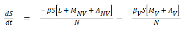
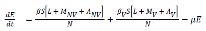
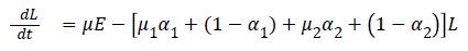
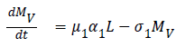
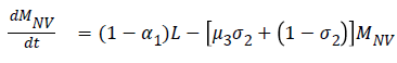
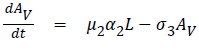
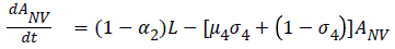
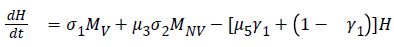
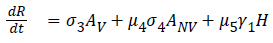
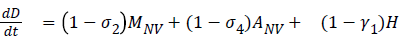
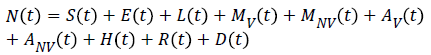
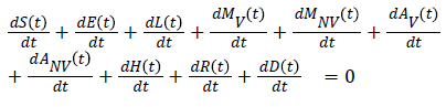
The model equations are listed below.
Stability of the disease free equilibrium
Consider the region:
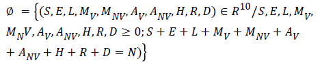
The given system has a disease free equilibrium given by U0=(N, 0, 0, 0, 0, 0, 0, 0, 0, 0). The linear stability of U0 is governed by the basic reproductive number (R0).
The stability of this equilibrium will be investigated using the next generation operator.
Here
X=(S, R),
Y=(E),
Z=(L,MV, MNV, AV, ANV, H, D)
(g ̃) (X*, Z)=β [L+MNV+ANV]+(βV S [MV+AV])/μ
Then M=β and D=μ1 α1+(1-α1)+μ2 α2+(1-α2)
Hence R0, the basic reproductive number=MD-1=β/(μ1α1+ (1- α1)+μ2α2+ (1-α2))
R0 is the reproduction number. If R0<1, the infection dies out and if R0>1 the disease spreads.
Theorem I
If R0<1, the disease free equilibrium of the given system is locally asymptomatically stable and unstable when R0>1.
1. The next generation operator approach: R0 is often found through the study and computation of the Eigen values of the Jacobian at the disease- or infectious-free equilibrium. Diekmann et al. follow a different approach: the next generation operator approach. They define R0 as the spectral radius of the “next generation operator". The details of this approach are outlined in the rest of this section. First, we consider the case where heterogeneity is discrete, that is, the case where heterogeneity is defined using groups defined by fixed characteristics, that is, for epidemiological models that can be written in the form:
dX/dt=f (X, Y, Z),
dY/dt=g (X, Y, Z),
dZ/dt=h (X, Y, Z),
Where X IRr, Y IRs, Z IRn, r, s, n ≥ 0, and h (X, 0, 0)=0. The components of X denote the number of susceptible, recovered, and other classes of non-infected individuals. The components of Y represent the number of infected individuals who do not transmit the disease. The components of Z represent the number of infected individuals capable of transmitting the disease.
Let U0=(X*, 0, 0) IRr+s+n denote the disease-free equilibrium, that is,
F (X*, 0, 0)=g (X*, 0, 0)=h (X*, 0, 0)=0
Assume that the equation g (X*, Y, Z)=0 implicitly determines a function Y=(g ̃ X*, Y). Let A=Dz h (X*, (g ̃X*, Y), 0) and further assume that A can be written in the form A=M-D, with M ≥ 0 (that is, mij ≥ 0) and D>0, a diagonal matrix.
The basic reproductive number is defined as the spectral radius (dominant eign value) of the matrix MD-1, that is,
R0=p (MD-1)
Theorem II
The disease free equilibrium of the given system is globally asymptomatically stable and unstable when R0<1.
2. Global stability conditions for the disease-free equilibrium
When R0<1 the disease-free equilibrium is locally asymptotic stable whenever R0<1 and unstable (LAS). When R0>1. Now, we list two conditions that if met, also guarantee the global asymptotic stability of the disease-free state. First, System 1.1 must be written in the form:
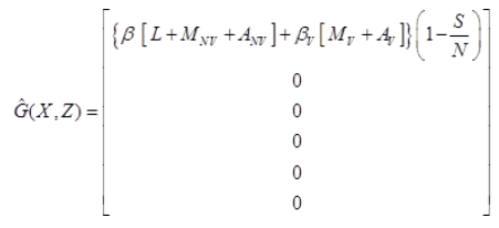
dX/dt=F (x, Z),
(2.1) dZ/dt=G (X, Z), G (x, 0)=0,
Where X IRm denotes (its components) the number of uninfected individuals and Where Z IRn denotes (its components) the number of infected individuals including latent, infectious, etc. U0=x0, 0 denotes the disease-free equilibrium of this system.
The conditions (H1) and (H2) below must be met to guarantee local asymptotic stability.
(H1) for dX/dt=F (X, 0), X* is a Globally Asymptotic Stables (GAS),

where A=Dz G (X*, 0), is an M-matrix (the off diagonal elements of A are nonnegative) and is the region where the model makes biological sense.
If System 2.1 satisfies the above two conditions then the following theorem holds:
Theorem: The fixed point U0=(x*, 0) is globally asymptotic stable equilibrium of 2.1 provided that R0<1 (LAS) and that assumption (H1) and (H2) are satisfied.
Proof
Let X=(S, R),
Z=( E, L,MV, MNV, AV, ANV, H, D),
F (X, 0)=(0) and
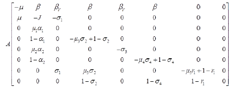
Where J=μ1 α1+(1-α1)+μ2 α2+(1-α2) and
Since, 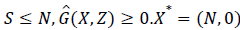 is globally asymptomatically stable for the system dX/dt=F (X, 0).
Also the off-diagonal elements of A are nonnegative i.e. A is an M-matrix.
Then the disease free Equilibrium of the given system is globally asymptomatically stable for R0<1.
Multi-hidden layer neural network with nonmultiplier
Hidden layer activation functions: Hidden layer h11 and h12: Knowing just the numbers of cases of infection identified by surveillance activities is not sufficient to identify the risk (probability) of infection occurring in the facility residents; rates must be used. Rates measure the probability of occurrence in a population of some particular infection. An incidence rate is typically used to measure the frequency of occurrence of new cases of infection within a defined population during a specified time frame (Figure 2).

Figure 2: Multi-hidden layer neural network with non-multiplier.
α1=(Symptomatic infected)/Susceptible
α2=(Asymptomatic infected)/Susceptible
Where,
α1=Symptomatic infection rate
α2=Asymptomatic infection rate
Hidden layer h13: Infected individual can transfer the disease with the respect to the contact rate, if there is any contact between the infected one with other susceptible, then the first individual infects the susceptible. Whether or not a particular kind of contact will be effective depends on the infectious agent and its route of transmission. The effective contact rate (denoted β) in a given population for a given infectious disease is measured in effective contacts per unit time. This may be expressed as the total contact rate (the total number of contacts, effective or not, per unit time, denoted γ), multiplied by the risk of infection, given contact between an infectious and a susceptible individual. This risk is called the transmission risk and is denoted p. Thus:
β=γ × ρ
The total contact rate, γ, will generally be greater than the effective contact rate, β, since not all contacts result in infection. That is to say, p is almost always less than 1 and it can never be greater than 1, since it is effectively the probability of transmission occurring.
Where,
β=Contact rate (Transmission rate), γ=Total contact rate and ρ=Transmission risk
p=(Total number of infected )/(susceptible)
Total number of infected=Number of symptomatic+Number of asymptomatic
γ=(Contact )/(Time )
Hidden layer h14 and h15
The disease may be transmitted from objects, but is most often transmitted by direct skin-to-skin contact, with a higher risk with extended contact. Initial infections require one to two weeks to become symptomatic.
μ1=(Distance )/(Symptomatic time)
μ2=(Distance )/(Asymptomatic time)
Where,
μ1=Velocity of latent people become symptomatic
μ2=Velocity of latent people become asymptomatic
Hidden layer hi

We used logistic activation function in the 2nd hidden layer with different learning rate ui.
Summation layer ε
Reproductive number R0=β/(μ1 α1+(1-α1)+μ2 α2+(1-α2)
R0 is the reproduction number. If R0<1, the infection dies out and if R0>1 the disease spreads. Tables 2 and 3 depict the training set and transmission rates for the proposed model respectively.
| Symptomatic infected | 0.4 | Hidden layer | Learning rate ui |
|---|---|---|---|
| Asymptomatic infected | 0.2 | μ1 | 0.5 |
| Susceptible | 0.8 | μ2 | 0.2 |
| Contact | 0.4 | Β | 0.0001 |
| Distance | 0.2 | α1 | 1.0 |
| Symptomatic time | 0.5 | α2 | 2.0 |
| Asymptomatic time | 0.2 |
Table 2. Training set.
| Iteration | μ1 | μ2 | β | α1 | α2 | R0 | Error |
|---|---|---|---|---|---|---|---|
| 1 | 2.0302 | 5.0302 | 1.0 | 1.0302 | 0.5000 | -0.0043 | 0.0043 |
| 2 | 2.1311 | 5.0065 | 1.0 | 1.3569 | 1.1065 | 0.0020 | -0.0020 |
| 3 | 2.1187 | 5.0067 | 1.0 | 1.2575 | 0.8307 | -0.0013 | 0.0013 |
| 4 | 2.1202 | 5.0067 | 1.0 | 1.2844 | 0.9340 | -0.0032 | 0.0032 |
| 5 | 2.1202 | 5.0067 | 1.0 | 1.2844 | 0.9340 | -0.0032 | 0.0032 |
| 6 | 2.1200 | 5.0067 | 1.0 | 1.2768 | 0.8930 | -0.0020 | 0.0020 |
| 7 | 2.1200 | 5.0067 | 1.0 | 1.2789 | 0.9094 | -0.0023 | 0.0023 |
| 8 | 2.1200 | 5.0067 | 1.0 | 1.2783 | 0.9028 | -0.0022 | 0.0022 |
Table 3. Training multi-hidden layer neural network.
Conclusion
The proposed SELMAHRD (Susceptible, Exposed, Latent, Symptomatic, Asymptomatic, Hospitalized, Recovered and Death) model will provide the number of hospitalized and number of death information for the policy makers to develop the prevention policies (Figure 3). The assumptions are similar to those of SIR model, which include total population is fix, population structure is not considered in the model, latent period will not change with time, and recovered people will not get infected again. In the model, infected are divided into two compartments i.e. latent and symptomatic. Some people may actually infect other people without any symptom, but later on their symptoms come out. According to the assumption, the vaccinated people directly go to the recovered compartment. This model explains the common ways to prevent influenza i.e. isolating susceptible people, letting them at home. Based on the SIR model, a more number of models developed for epidemic diseases such as SIRS, SEIR, SEIRS, SEIRD, SEIAHR, SELMAHRD etc. SELMAHRD model might not provide vaccinated and non-vaccinated people behaviours. In proposed model, susceptible have two kinds of people, they are vaccinated and non-vaccinated. We assume that vaccinated will not die due to disease. The proposed compartmental epidemic model is used to calculate the basic reproduction number R0 and dynamics of disease-free equilibrium for influenza A (H1N1) in Vellore, Tamil Nadu, India. However, the realistic details of transmission cannot be determined from such models. Hence, multi-hidden layer neural network with nonmultiplier is used to elucidate other factors that also influence the disease dynamics. We conclude that the transmission of influenza A (H1N1) in Vellore, Tamil Nadu, India is under control and can be totally eradicated if the number of Government authorized H1N1 treatment centers are increased and the supply of drugs to these centers could be increased.

Figure 3: Simulation of SELMiAjHRD model.
References
- Kermack WO, McKendrick AG. A contribution to the mathematical theory of epidemics. Proc Royal Soc 1927; 115: 700-721.
- Sze BH, Ying HH. On the role of asymptomatic infection in transmission dynamics of infectious diseases. Bull Math Biol 2008.
- Kang H, Jin YH. A new SIR-based model for influenza epidemic. W Acad Sci Eng Technol 2012; 67.
- Bimal KM, Aditya KS. SIjRS E-epidemic model with multiple groups of infection in computer network. Int J Nonlin Sci 2012; 13: 357-362.
- Van den Driessche P, James W. Reproduction numbers and sub-threshold endemic equilibria for compartmental models of disease transmission. Math Biosci 2002; 180: 29-48.
- Phenyo EL, Barbel FF. Statistical inference in a stochastic epidemic SEIR model and with control intervention: Ebola as a case study. Biometr 2006; 62: 1170-1177.
- Tim L, Megan J, Cody C, Ozgur MA, John WF. Simulating pandemic influenza preparedness plan for a public university: A hierarchical system dynamics approach. Proc Winter Simul Conf 2008; 70: 134-155.
- Castillo CC, Feng Z, Huang W. On the computation of Ro and its role on. Mathematical approaches for emerging and re-emerging infectious diseases: an introduction ADS Phys Serv 2002; 1: 229.
- Van den Driessche P, Watmough J. Further notes on the basic reproduction number. Math Epidemiol 2008; 159-178.
- Diekmann O, Heesterbeek JAP, Metz JAJ. On the definition and the computation of the basic reproduction ratio R0 in models for infectious diseases in heterogeneous population. J Math Biol 1990; 28: 365-382.
- Zhien M, Yicang Z, Jianhong W. Modelling and dynamics of infectious diseases, higher education press-China. W Sci Publ Co Singap 2009.