Research Article - Environmental Risk Assessment and Remediation (2017) Volume 1, Issue 3

Improving grid-connected PV dc yields obtained with daily models.

Amin Bennouna^*, Noura Aarich, Noureddine Erraissi, Mohamed Akhsassi and Mustapha Raoufi

Department of Physics, Faculty of Science Semlalia Marrakech, Cadi Ayyad University, Morocco

*Corresponding Author:

Amin Bennouna
Cadi Ayyad University
Morocco
Tel: +86-13615286708
E-mail: sindibad@uca.ma

Accepted date: July 20, 2017

Abstract

This work is part of the "PROPRE.MA" project which main goal consists on drawing gridconnected photovoltaic yield maps for all Morocco with ground calibration using identical plants installed in partner institutions located in 20 different Moroccan cities. To have monthly calibration corrections as small as possible, the monthly maps before calibration must be as realistic as possible, and above all, the calibration factors undergo the least possible temporal and spatial variations. From an investor perspective, the specific energy yield is the most important parameter since it has and immediate effect on the levelized cost of electricity (LCOE), with all its impacts. In this paper, we estimate expected monthly averages of daily energy yields with methods which use solar maps published by weather services dedicated to solar energy. We present a comparison of monthly averages of PV daily yields calculated with our own models as well as with values obtained from international databases. In terms of methodology, our paper refers always to the results of an hour-by-hour simulation software. Whatever picture we take, we find that linear “simple models” tend always to overestimate yields and we explain why. We propose a non-linear model which seems to be the best compromise for our future PV yields database.

Keywords

Photovoltaic grid-connected systems; photovoltaic yields models; monthly average of daily dc yields; yearly dc yields; comparison of photovoltaic yields; Morocco.

Introduction

Frame of the present work

Morocco should be adopting very soon the net-metering approach for low-voltage grid-connected photovoltaic plants. In this view, installation over-sizing becomes critical for the investor since the electricity distributor is not supposed to buy the feed-in energy surplus at the end of a given period (monthly being the smallest). In these conditions, it is critical to know the amount of PV solar electricity generated at any specific Moroccan location at least, at the monthly level.

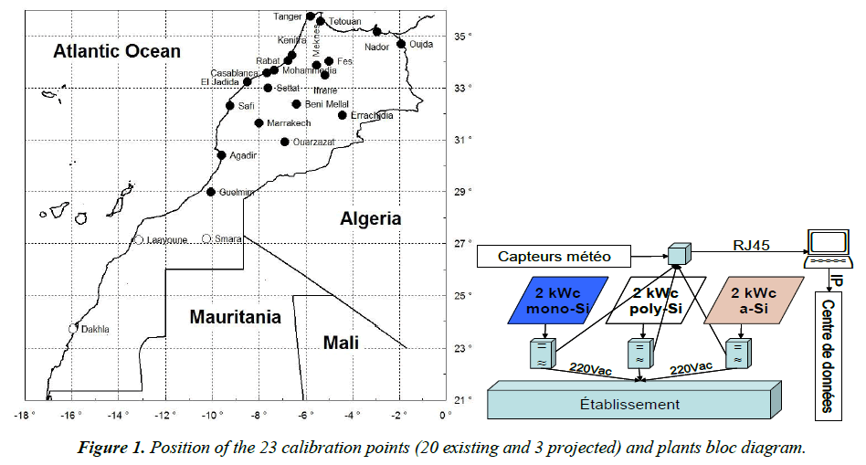
This work is part of the "PROPRE.MA" project (www.propre. ma), sponsored by IRESEN (02/2014-01/2016), proposed and leaded by the Faculty of Science Semlalia Marrakech and conducted by 20 Moroccan higher education institutions and “RESING”, a private company. The main goal of "PROPRE. MA" consists on drawing grid-connected photovoltaic yield maps for the whole country with ground calibration using identical plants installed in partner institutions located in 20 different Moroccan cities shown in Figure 1. Each plant consists on a 2-kWp array of each of the three silicon PV module technologies: crystalline, polycrystalline and amorphous, as shown in Figure 1. The global scope of the project consists on drawing acceptable resolution PV yields maps properly calibrated with actual ground measurements.

Figure 1. Position of the 23 calibration points (20 existing and 3 projected) and plants bloc diagram.

Calibration should take place by the second half of 2015, after a one-year measurements period. For the maps, 1192 appropriate representative points have been already selected in throughout all Morocco. To have monthly calibration corrections as small as possible, the monthly maps before calibration must be as realistic as possible, and above all, the calibration factors undergo the least possible temporal and spatial variations.

Goal of the present work

Presently, to get the dc yield of a grid-connected photovoltaic plant, one has to choose between:

- applying a “simple model” using monthly averages of temperature and of daily horizontal solar radiation on facing south tilted modules, with easy handling on a single spreadsheet line but with reduced precision,

- running an external hourly dynamic program, with a better precision but heavy drawback to handle 12 times (months) for each of the 1,192 points of the map.

We have chosen an intermediate solution consisting on a compromise between both improving the precision of the first “simple model” by finding correlations of its PV yields and those obtained by an hourly dynamic program.

The “corrected simple model” so designed is supposed:

- to use no more input data than the daily models (daily temperature and horizontal solar radiation),

- to be generated by an on-site database query for each of the 1,192 data lines.

Bibliographical overview

We have found 15 reviews of the state-of-the-art in PV performance calculation methods [1-15] and no less than 49 papers dedicated to several aspects of the topic of this paper, and among them:

- 04 propose methods for short term forecasting of PV yields [16-19],

- 04 deal with elements for Geographical Information Systems [20-23],

- 11 proposed models for PV performance [24-34],

- 07 proposed models for PV performance with experimental validation [35-41],

- 14 have done PV systems monitoring [42-55], including systems comparison,

- 03 have simulated the PV operation or performance with existing software [56-58],

- 06 have considered some other aspects than our major concern of this paper [59-64].

In the “PROPRE.MA” project, we will have to deal with almost all this aspects. For what concerns this same paper, the first authors1 classified methods for energy harvesting calculation of PV generators in two groups:

- those that directly calculate the energy,

- those that indirectly calculate the energy from the power, these divide again in two categories:

• those that directly calculate the power.

• those that indirectly calculate the power from the I-V curve.

Here, we will use at least one of each of these groups and categories which, of course, differ in simplicity and accuracy and we will choose the most suitable method for our specific application.

Fundamental background

Approach of the problem

We will call here “linear models” those that give results proportional to the solar irradiance in instantaneous or to the received global solar radiation during a given period (day, month or year).

At a given cell temperature, even if the short circuit current is directly proportional to the solar radiation intensity, the opencircuit voltage shows a non-linear behaviour against the solar radiation intensity and consequently, the maximum power also. The things become more complex when considering variations of ambient temperature, its impact on the cell temperatures and therefore, in the output power. The two following graphs illustrate our following argumentation [65-67].

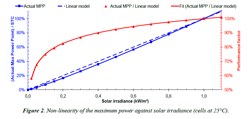
Maximum power against solar irradiance is non-linear because of the complex shape of current-voltage characteristic. In addition, its non-explicit character excludes any analytic direct calculation. Figure 2 was calculated from data obtained with PiViDyn software (described below in the subchapter 2.4) for cells maintained at 25°C. It shows:

- the actual relative maximum power point (blue squares and left scale) which has to be compared to the linear model (dotted blue and line left scale) with which it should match when excluding non-linear effects,

- the performance factor, ratio of the actual power and the linear model (red triangles and right scale) which highlights the importance of the relative mismatch between them.

The same type of curve could be obtained from parameters either:

- derived from the data sheet information of PV modules,

- from modules current-voltage characteristics at difference irradiance levels.

Figure 2 highlights clearly the effects arising from the nonlinearity of voltage against solar irradiance, even at constant cells temperature.

Figure 2 shows also that the performance factor (PF) for cells kept at 25°C (red triangles in Figure 2) is very well correlated by the intuitive formula (red solid line in Figure 2), valid above 0.04 kW/m² and forced to pass through the point (1, 1):

Figure 2. Non-linearity of the maximum power against solar irradiance (cells at 25°C).

PF(θ_c=25°C) = [1 + C_m . L_n(I_solar / I_STC)]

Where,

- I_solar and I_STC, both expressed in the same unit, are actual and STC (1,000 W/m²) solar intensities,

- C_m is a constant depending on module technology (found near to 0.10925 for the crystalline silicon module concerned here).

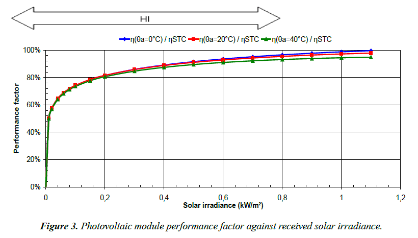
For various ambient temperatures, Figure 3 shows the performance factor of a module against solar radiation intensity. It was calculated with the absolute efficiency η obtained with PiViDyn software (described below in the subchapter 2.4) forcing the data with the given ambient temperatures (0°C, 20°C and 40°C).

Figure 3. Photovoltaic module performance factor against received solar irradiance.

Beside the values shown in this figure, which may vary from a manufacturer to another, our argument hereafter is essentially with the shape itself of the curves shown in Figure 3:

- all the early mornings and late afternoons of all the year, solar radiation intensity lies in the zone “LO” of the curves, below 0.2 kW/m² where PV module efficiency rises sharply from zero,

- in the middle of the days, solar radiation intensity lies in the zone “HI” of the curves, above 0.2 kW/m² where PV module efficiency varies slowly with solar irradiance intensity and almost linearly.

Typically, a day with:

- a high PV yield is a day for which during most of the day, the modules have operated in the “HI” zone, with a reduced energy impact of early mornings and late afternoons,

- a medium PV yield is a day for which the energy impact of early mornings and late afternoons is not negligible,

- a low PV yield is a day for which the energy impact of early mornings and late afternoons is very important,

Therefore, at the end of a given day, the impact of non-linear effects on electric energy generated will vary from negligible (for very sunny and long days) to substantial (for not very sunny or short days). Consequently, the impact of the low solar intensity on the daily photovoltaic yield increases when daily received solar energy decreases, therefore for low yield days. At the bottom line, linear models overestimate the actual yields.

Our idea, and scope of part of this paper, is to estimate this impact and adjust a daily yield “simple model” based on the values of the daily yield “simple model” themselves.

Overview of a “simple model” (SM)

Basics of the “simple model” (SM): Photovoltaic DC yields obtained with a “simple model” need monthly averages of temperature and of daily solar radiation on fixed tilt modules. In such conditions, photovoltaic DC yields can be easily calculated inside a database by an on-site query from the input data in the same line.

The “simple model” we propose to adjust is the monthly average of the daily DC PV yield <y_SMi> (in Wh/Wp.day) which is given by:

<y_SMi> = (Gβi / I_STC). (1-α_p)^(<θci>-25), where

? α_p is the temperature coefficient of power (set at 0.295%/K to match with PiViDyn values); we would like to point that the exponent shape of the rightmost term is the exact solution of the differential equation (dP/dθ) = α_p.P with the power condition P=P_STC at 25°C, even if the linear approximation of the solution is more popular,

? Gβi (in Wh/m².day), is the global daily radiation falling on a facing south surface, tilted at an angle β (30° in our case), for a typical day of the month i. Gβi was calculated from the horizontal radiation Hi using an algorithm described in reference which background refers essentially to reference,

? I_STC is the solar intensity under STC conditions (1.000 W/m² or 1 when Gβi is expressed in kWh/m².day) and (Gβi / I_STC) represents the number of peak hours in the day i, equivalent of hours at 1 kW/m²,

? <θ_ci > is the daily average of cell temperature (in °C) for a typical day i, given by:

θci> = < θai> + <I_βi> . (NOCT-20) / 800, where

• <θai> is the daily average of ambient temperature for a typical day of the month i,

• NOCT, the normal operating cell temperature (set at 47°C to match with PiViDyn values),

• <I_βi> is the daily average of solar radiation intensity Iβi (in W/m²), used to distinguish between days having the same solar radiation with different durations (e.g. different average solar radiation intensities) and given by:

<I_βi> = Gβi / Di, where

• Di is the length of the day i (in hours), given by:

Di= (2/15). Arc cos (-tg δi . tg φ), where

• δi is the solar declination for the typical day i

• φ is the latitude of the site.

Thermal legitimacy of using the daily average temperature: To justify the replacement of the instantaneous values of θci and Iβi by their daily averages <θci> and <I_βi>, we show here below the experimental results obtained by other authors in the island of Crete.

From the slope of the straight line of Figure 4 (0.0332°C.m²/W), it is easy to extract the Normal Operation Cell Temperature (NOCT at 45.8°C) which is perfectly compatible with common values for crystalline silicon modules like the ones used by the authors. It is then legitimate to use the monthly averages of temperature and of daily solar radiation intensity, at least from the thermal point of view. From the electrical point of view, things are different because of non-linear impact on the current.

Figure 4. Summary of data collected from reference69 (left) and calculations done with them (right).

Crucial comments on the “simple model” (SM): The main problems of models like the “simple model” we presented here above are that:

- they are not sensitive to the specific module electrical characteristics, even if the module thermal properties are present through the NOCT value in the formula,

- they represent an overestimation of the real photovoltaic yields, simply because of the shape of the output power shown in Figure 2 and the comments that follow it.

Overview of a “non-linear model” (NLM)

This model carries such a name because the performance factor:

- uses the logarithmic behavior used for Figure 2,

- is corrected for temperature before even the application of the related formula:

PF(θc) = {1 + C_m . L_n[(I_solar / I_STC).(1-α_p)^(<θci>-25)]}

The non-linear photovoltaic yield is then given by:

<y_NLi> = (G_βi / I_STC).{1 + C_m . L_n[(<I_βi> / I_STC).(1-α_p)^(<θci>-25)]}

Here, the temperature correction has been directly applied to (<I_βi> / I_STC) because correction outside the brackets failed to give satisfying results. In fact, its coherence resides in the fact that solar intensity “acts as a lower value” when cell temperature increases with respect to STC conditions (25°C).

The advantage of models like the “non-linear model” we presented above is that they take into account the module electrical characteristics as well as its thermal properties and, as for the simple model, they can be easily calculated inside a database by an on-site query from the input data in the same line [68-70].

Overview of the instantaneous dynamic simulation program “PiViDyn” (PVD)

PiViDyn meteorological database: The program includes a database of 2.200 sites for which horizontal solar radiation and temperature are available. It also allows bypassing automatic reading from the database through a manual entry of latitude, as well as monthly averages of temperatures and of horizontal solar radiation. This is the way we adopted to include the following meteorological data:

- “Meteonorm” data [70,71] , taken from PVSyst software, for 24 sites

- "SOLEMI & Helioclim-3" data, downloaded from Solar Med Atlas website, for 20 sites

- "Climate-SAF PVGIS" data, downloaded from PVGIS website, for 24 sites

- "NASA Surface meteorology and Solar Energy Data Set" data (NASE-SSE), taken from RETSCREEN Software for 24 sites.

We have multiplied the sources of data because we intend to validate the fact that our final adjustments are independent on the meteorological input data.

PiViDyn model of the hourly solar radiation intensity: The global irradiance Isolar falling on a surface azimuthally oriented at s and tilted at β is given by:

I_solar = I_direct + I_diffuse + I_albedo, where

I_direct, I_diffuse and I_albedo are respectively the direct, the diffuse and the albedo component of the received irradiance on the tilted surface. To avoid unnecessary lengthening this paper, we will simply note that the various components are obtained with standard methods to get solar irradiance from the horizontal radiation alone [68], through the Collares-Pereira correlative method.

PiViDyn model of the hourly ambient temperature: In the model used, not valid by night, the minimum ambient temperature is at sunrise at (12 - Di / 2) solar time while maximum is in mid-afternoon (12 + Di / 4). The daily average ambient temperature is:

<θ_ai> = (θ_max + θ_min) / 2, where

θ_max and θ_min are the daily maximum and minimum temperatures, and temperature amplitude is given by:

Amp = (θ_max - θ_min)/2

Then, the model used for the diurnal variation of temperature is:

θ_a(t) = <θ_ai> + Amp . cos{[2π/(3D_i/2)].[t – (12+D_i/4)]}

PiViDyn calculation of the current-voltage characteristic: At each instant, the calculation program divides an expected open circuit voltage Voc in 100 intervals and solves iteratively the following current (I)-voltage (V) equation for one cell:

I = I_SC - I_S.{exp{q.[V - R_S.I] / [n.kT_c]}-1} – [V - R_S.I] / R_sh,

where

T_c is the cell absolute temperature (in K), given by:

T_c = (θ_a + 273.16) + I_solar.(NOCT - 20)/800, where

I_solar is the solar radiation intensity in (W/m²)

θ_a is the ambient temperature in (°C)

NOCT is the Normal Operation Cell Temperature (in °C, set here at 47°C in our case)

I_SC is the short circuit current depending on the cell temperature, given by:

I_SC(T_c) = S_ph(25°C).S_c.I_solar.[1 + α_I.(T_c - 298)], where

S_ph(25°C) is the photoelectric sensibility factor at 25°C (set here at 2.10-5 A/W)

S_c is the surface of the cells in series in the module

α_I is the temperature coefficient of current (set here at +0.063%/K)

I_S is the saturation current depending on the cell temperature, given by:

I_S(T_c) = J_s(25°C). S_c.[1 + α_I.(T_c - 298)], where

J_s(25°C) is the saturation current density at 25°C, given by:

J_s(25°C) = ρ_S(25°C) / [8000.R_sh(25°C)], where

ρ_S(25°C) is the series resistivity at 25°C (set here at 75 Ω.C_m)

R_sh(25°C) is the shunt resistance at 25°C (set here at 40,000 Ω)

R_S is the series resistance depending on the cell temperature, given by:

R_S(T_c) = ρ_S(25°C).e. [1 + α_I.(T_c – 298.16)] / S_c, where e is the cell thickness

Rsh is the series resistance depending on the cell temperature, given by:

R_sh(T_c) = R_sh(25°C). [1 + α_I.(T_c - 298)]

n is the ideality factor and is supposed to vary with cell temperature like

n(T_c) = n(25°C).{1-(|α_I| + |α_V|)].(T_c - 298)}, where

α_V is the temperature coefficient of voltage (set here at -0.358%/K)

q is the charge of the electron and k the Boltzmann constant

For more precision at the beginning and end of the day, the program also corrects the solar radiation intensity Isolar for the variation of the glass optical reflectance with respect to its value at normal incidence, for which the modules properties are valid. This is done applying the Fresnel transmittance laws to the glass and normalizing them to the normal incidence value [69-75].

A result of the PiViDyn program: Results shown in Figure 5 were obtained using PiViDyn program. It shows the yearly evolution of the daily average performance factor of a crystalline silicon solar module, calculated in several sites for modules facing south and tilted at the latitude of the site. The results confirm what we have anticipated from Figure 3: the difficulty to find an a priori yield daily model valid for all seasons, especially when the average performance is lower.

Figure 5. Performance factor of a crystalline silicon solar module.

Given the abscissa scale, it is true that, variations are not huge for a single site but they are worth taking into consideration when a better precision is required.

Calculations

Sites considered in this work

In Table 1, the 20 first cities are the ones for which the Moroccan photovoltaic monthly yield maps will be calibrated. We have added to them the 4 subsequent European cities to get few points in the tail of low monthly averages of daily PV yields because we did not find at any season in almost all Morocco below 3.2 Wh/Wp.day at 30° tilt.

Table 1. Cities concerned by the calculations of the present work.

Sources of meteorological data, of external PV yields and calculations done

As shown by Table 2:

Table 2. Different input and output data considered for the present work.

? from each of the four sources (PVS, SMA, PVG and RTS) we have:

? extracted the meteorological data,

? taken from databases the PV yields (SMA and PVG) or calculated them with the related software (PVS and RTS).

? with each of the four meteorological data sources (PVS, SMA, PVG and RTS), we have calculated PV yields with:

? the PiViDyn program,

? the simple model (SM),

? the non-linear model (NLM).

Simple model (SM) and its modified version (MSM)

PV yields from PVS, SMA, PVG and RTS against the simple model PV yields (SM):

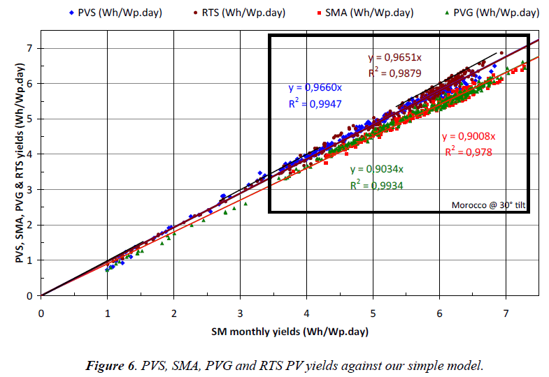
Figure 6 shows:

Figure 6. PVS, SMA, PVG and RTS PV yields against our simple model.

- the PV yields calculated with PVSyst Software (blue diamonds) against our SM calculated with the same metrological data,

- the PV yields taken from Solar Med Atlas (red squares) against our SM calculated with the same metrological data,

- the PV yields taken from PVGIS (green triangles) against our SM calculated with the same metrological data,

- the PV yields calculated with RESTCREEN Software (brown circles) against our SM calculated with the same metrological data.

The first comment we would like to do is that almost all the data are proportional to our “simple model”. This means that, once divided by the coefficients shown in the graph (0.9660 for PVS, 0.9651 for SMA, 0.9034 for PVG and 0.9008 for RTS), one obtains normalized values PVS*, SMA*, PVG* and RTS* which are almost the same than our SM results.

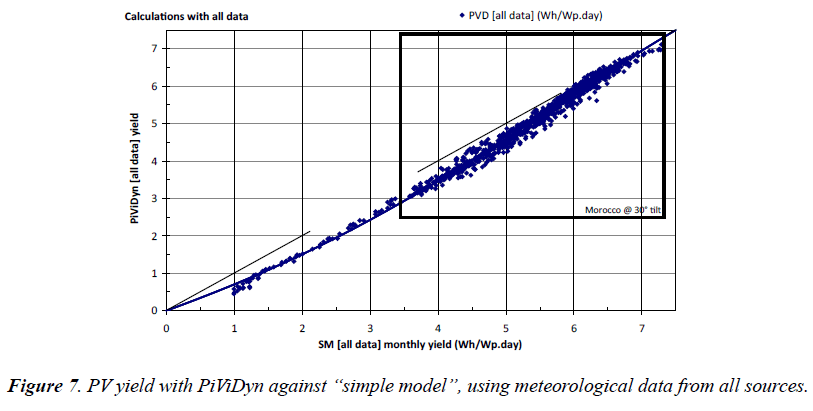
Hourly integrated PV yields (PVD) against the simple model PV yields (SM): Figure 7 shows the PV yields obtained with PiViDyn software against the “simple model” (SM, from subchapter 2.3), both calculated with the same meteorological data taken from all sources (PVS, SMA, PVG, and RTS).

Figure 7. PV yield with PiViDyn against “simple model”, using meteorological data from all sources.

Almost all points are below the dotted line of the first bisector.

The least squares method polynomial correlation represented by the solid line curve in Figure 7 will be used later. The correlation coefficient is 99.55%, despite the fact polynomial has no physical justification.

The shape of the solid line curve in Figure 7 reminds that of electric power in Figure 2 because the SM yield model is directly proportional to the daily-received solar radiation, which is the time integral of the abscissa of Figure 2. In agreement with comments in subchapter 2.2.3, the solid line curve must tend towards the bisector by lower values [76-78].

The dispersion of the points around the average solid line curve is simply due to the differences induced by the two estimation methods (hourly and daily).

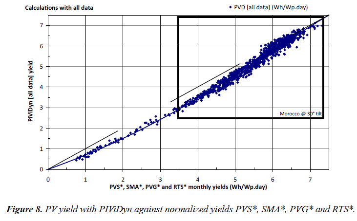
Hourly integrated PV yield (PVD) against the PV yields from PVS, SMA, PVG and RTS: Figure 8 shows the PV yields obtained with PiViDyn software (same ordinate than Figure 7 above), but this time against their normalized PV yields PVS*, SMA*, PVG* and RTS* (Figure 6). Almost all points are below the dotted line of the first bisector.

The solid line is the same than the one already shown in Figure 7. With the new abscissa, the same polynomial fits the PVD data with a correlation coefficient of 99.00%, which is still good enough to say that the nature of our simple model results (SM) is similar to the PVS, SMA, PVG and RTS yields.

Of course, the shape of the solid line curve in Figure 7 still reminds that in Figure 2 for the same reasons commented above.

Adjusting the simple model mismatch: modified simple model (MSM): In a preliminary presentation of our results, we have already used a polynomial correlation to adjust the yields for the first test maps. In this part of the work, we take here the same approach but improving it from several points of view:

- calculating with four times more meteorological data sources,

- expanding the values and the method to lower yields,

- using a higher degree polynomial than previously, but above all, which tends to the first bisector from lower values, in agreement with comments in subchapter 2.2.3, which was not the case in our previously mentioned communications [79,80].

The polynomial correlation forced to pass at the origin and obtained by the least squares method for Figure 7 and Figure 8 is:

Figure 8. PV yield with PIViDyn against normalized yields PVS*, SMA*, PVG* and RTS*.

<y_MSMi> = {a₄.<y_SMi>⁴ + a₃.<y_SMi>³ + a₂.<y_SMi>² + a₁.<y_SMi>}

<y_MSMi> = <y_SMi> .{a₄.<y_SMi>³ + a₂.<y_SMi>² + a₂.<y_SMi> + a₁}

<y_MSMi> = <y_SMi> . NLMF_i

with a₄ = -0.0008946, a₃ = 0.0086477, a₂ = 0.0302013 and a₁ = 0.6645285.

We have chosen this polynomial degree because higher or lower had all a tendency to cut the first bisector in the upper part of our yield window [7.5 Wh/Wps.Day], in contradiction with the need to reach the first bisector by lower values, in agreement with our comments at subchapter 2.2.3.

We call the term between brackets the “non-linear multiplicative factor” (NLMF_i), which is supposed to bring the simple model yields to more realistic values.

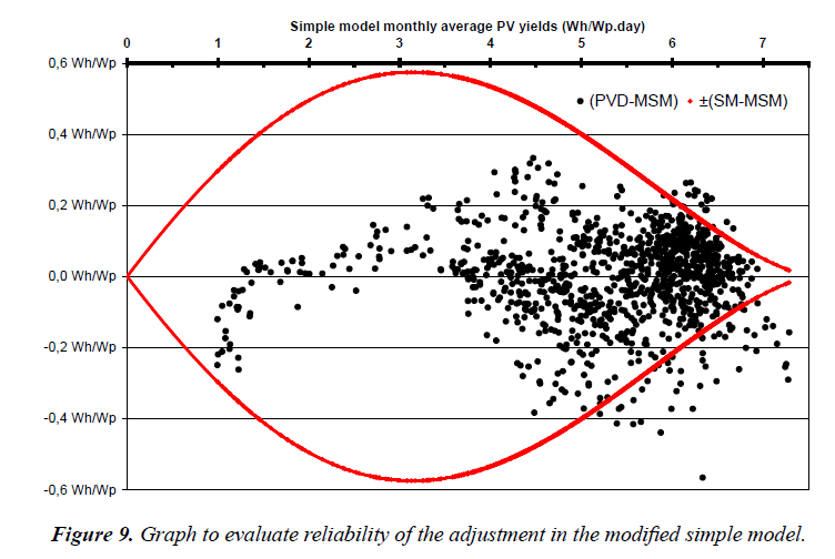
Reliability of the adjustment in the modified simple model (MSM): We may have to ask the question of the usefulness of such adjustment (in MSM) to such a dispersion of points around the polynomial fit in Figure 7 and Figure 8. The best way we found to give an answer to this is to compare the dispersion of the points around the average with the adjustment.

Figure 9 shows at the same time:

Figure 9. Graph to evaluate reliability of the adjustment in the modified simple model.

- the difference between PV yields obtained with PiViDyn software and those of the modified simple model (polynomial fit of subchapter 3.2.4),

- the difference between the simple model yields and the same the modified simple model yields (polynomial fit of subchapter 3.2.4).

At a given value of SM yields, the more points there are outside the curve, the more it is pertinent to make such an adjustment. With the amount of data we have, it seems like important to avoid using yields models like our SM without adjustment below 5-5.5 Wh/Wp.day. We are quite concerned with regard to our monthly yield maps, since the monthly averages of daily yields can drop to around 3.2 Wh/Wp.day with a tilt angle of 30° for several Moroccan cities.

We would like to draw attention to the fact that this is valid only for monthly averages of daily yields and not for their yearly averages, which, hopefully, can compensate and lead to smaller uncertainties (as we will see below).

It is true that, for simple model yields above 5.5 Wh/Wp.day, the dispersion of the points is as important (few percent) as the recommended multiplicative adjustment itself but, when having only the simple model values <y_SMi>, the adjustment is strongly recommended below 5.5 Wh/Wp.day.

At the bottom line, even without a physical justification, this empirical adjustment (NLMF) is a kind of “better than linear”.

PV yields obtained directly through the non-linear model (NLM)

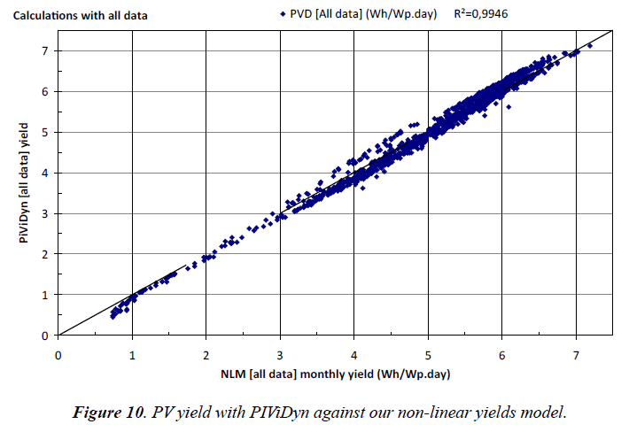
Hourly integrated PV yields (PiViDyn) against the non-linear model (NLM): Figure 10 shows the same PV yields obtained with PiViDyn software (same ordinate than Figures 7 and 8 above), but this time against their related PV yields calculated with our non-linear model (NLM, from subchapter 2.3).

Figure 10. PV yield with PIViDyn against our non-linear yields model.

This time, with the new abscissa, it is the first bisector dotted line which gives a correlation coefficient of 99.46%, meaning that the non-linear model (NLM) fits in a very good way the PiViDyn software calculations.

We found no explanation to the points that disperse more than the others do.

With think that, in the low monthly yields zone, the overestimation of the NLM (points below the first bisector) may come from a bigger impact of optical reflectance losses that are taken into account by the PiViDyn software while not by the NLM [80].

Non-linear multiplicative factor, NLMF: If we would like to take into consideration non-linear effects adjusting with a multiplicative factor (NLMF_i) for each month i, this is defined by:

NLMF_i = <y_NLi> / <y_SMi>

<y_NLi> / <y_SMi> = {1 + C_m . L_n[(<I_βi> / I_STC).(1-α_p)^(<θci>-25)]} / (1-α_p) ^(<θci>-25)

Such an expression does not depend explicitly and only on <y_SMi>. It gives the right analytical formula of what we have empirically expressed with a third degree polynomial in the subchapter 3.2.4.

Conclusions

We have done a few calculations with a different module tilt angle (60°) but, as expected, the new points fell in the same cloud than the ones shown above. This is because what we have done above concerns already cities with up to 24° difference in latitude, all seasons and a wide variety of received solar radiation ranging from 0.95 to 7.6 kWh/m².day.

As seen from the PROPRE.MA project point of view, it is crucial to conclude this paper with impacts on yearly yields.

Yearly yields for the 20 calibration cities in Morocco

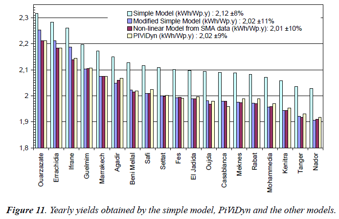
Comparison of yearly yields we calculated for this work: Figure 11 allows comparing the yearly yields obtained through different methods for each of the 20 Moroccan cities.

As shown in the Figure 11 legend, the global “country average” of yearly PV yields for the 20 cities, as calculated with Solar Med Atlas data stands around:

Figure 11. Yearly yields obtained by the simple model, PiViDyn and the other models.

- 2.12 kWh/Wp per year with ± 8% dispersion over the cities for the simple model,

- 2.02 kWh/Wp per year with ± 11% dispersion over the cities for the modified simple model,

- 2.01 kWh/Wp per year with ± 10% dispersion over the cities for the non-linear model,

- 2.02 kWh/Wp per year with ± 9% dispersion over the cities for PiViDyn.

It is clear that simple models tend to overestimate the photovoltaic yields obtained with and hourly software. MSM passage to NLM is not always in the same direction (decrease or reduce yield). At this stage, the choice between MSM and NLM does push us to the second as physical proof of its mathematical expression.

It is also quite satisfying to see how the NLM gives yearly yields very near to the PiViDyn software.

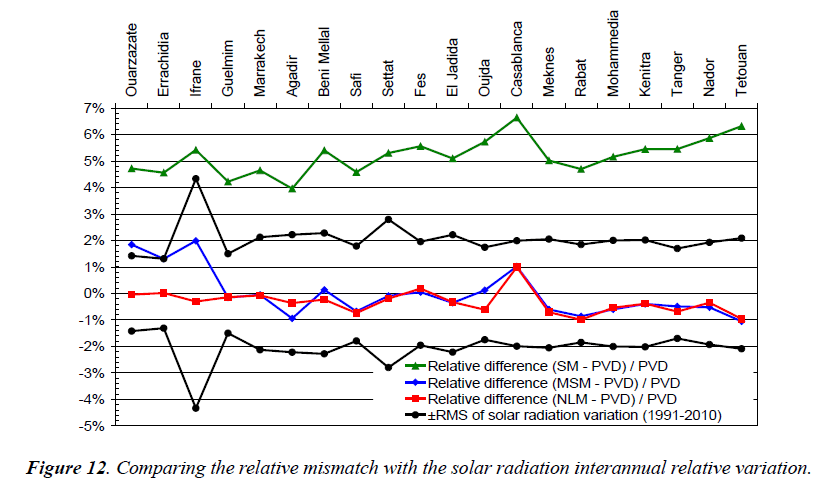
Impact of correcting the simple model instead of integrating hourly results: In a single graph, Figure 12 shows the relative difference to PVD yearly yields to:

Figure 12. Comparing the relative mismatch with the solar radiation interannual relative variation.

- the simple model yearly yields (SM-PVD)/PVD,

- the modified simple model yearly yields (MSM-PVD)/ PVD,

- the non-linear yearly yields (NLM-PVD)/PVD,

For the “PROPRE.MA” project, we are supposed to stay inside the root mean square of inter annual variation of solar radiation (1991-2010), which, in Figure 12 is verified by the MSM and NLM models. For the time being, we have no choice than choosing an hourly simulation as a reference (PiViDyn) and our exigency excludes evidently the use of the simple model or any other similar.

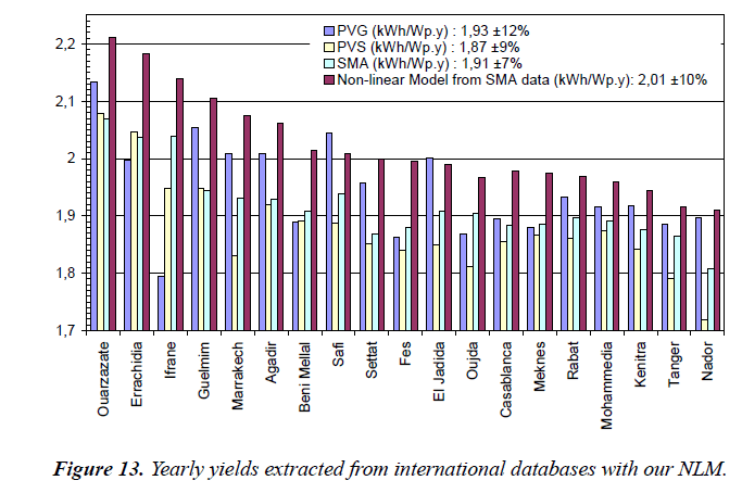
Comparison of our NLM yearly yields with other sources: For each of the same above 20 Moroccan cities, Figure 13 allows comparing the yearly yields obtained with our NLM with other sources.

Figure 13. Yearly yields extracted from international databases with our NLM.

Figure 13 legend, shows that the global “country average” of yearly PV yields for the 20 cities is around:

- 1.93 kWh/Wp per year with ± 12% dispersion over the cities for PV-GIS database and 4.8% less, in average, than our NLM,

- 1.87 kWh/Wp per year with ± 9% dispersion over the cities for the PV-Syst software and 7.0% less, in average, than our NLM,

- 1.91 kWh/Wp per year with ± 7% dispersion over the cities for the Solar Med Atlas database and 5% less, in average, than our NLM

- 2.01 kWh/Wp per year with ± 10% dispersion over the cities for our non-linear model (calculated with the above Solar Med Atlas meteorological data).

Even calculated with the same meteorological data, the yearly PV yields “country average” calculated with our NLM is about 5% higher than the value given by Solar Med Atlas.

Main conclusion

As seen from now, when comparing our own models together, the more reasonable chose should be to go with the non-linear model, which should allow direct access to technologically dependent monthly yields for the next steps (see subchapter 4.3) and being, at the same time, generated by on-site database query.

It is also evident that external sources yearly yields are more “conservative” (from 3.7 to 7% less in average of annual values) than those obtained with our NLM. Only our future ground calibration will tell us which is the more realistic. Hopefully, the differences are small enough for not changing any investment strategic decision in grid-connected PV in Morocco but 3.7 to 7% can affect slightly long term business planning, especially that the difference can be locally bigger than this. But it is obvious that this last may play a significant role for long term purchase contracts 7% less in energy output forecast can change a tender winner.

At this point, we think having proven that, if a yearly calibration is sufficient for feed-in-tariff solar investors, it might be not sufficient for the net-metering when the monthly values of photovoltaic yields are required.

Next steps

Before receiving the calibration data and going to the calibration phase, we will have to do the same type of work done here above to elaborate the same type of data for polycrystalline and amorphous silicon, specially, because the NLM shows a dependence on C_m (constant depending on module technology) and α_p (module power temperature coefficient). It is too early to evaluate the final impact of changing the module technology but we can guess that it should be small, even if not negligible.

Acknowledgements

In the name of all consortium members, authors would like to thank IRESEN Board and Scientific Committee for financing this through the INNO’PV Program as well as its General Manager, Badr IKKEN, and the management & operations staff for their daily efforts with the “PROPRE.MA” project.

Among the last steps of this project, ground calibration is far from being the less important and it would not be achieved without the contribution of all the other partners of the “PROPRE. MA” project, namely (Institution acronym and city, University acronym), in city alphabetic order: Ahmed IHLAL (F.S. Agadir, U.I.Z.), Mustapha MABROUKI (F.S.T. Beni Mellal, U.S.M.S.), Abderraouf RIDAH (F.S. Casablanca Ben Msik, U.H2.M.), Mohammed KHAIDAR (F.S. El Jadida, U.C.D.), Abderrazak LFAKIR (F.S.T. Errachidia, U.M.S.), Izeddine ZORKANI (F.S. Fes, U.S.M.B.A.), Abdeslam EL FANAOUI (E.S.T. Guelmim, U.I.Z.), Khalid LOUDIYI (S.S.E. Ifrane, A.U.I.), Mounir FAHOUME (F.S. Kenitra, U.I.T.), Mustapha RAOUFI (F.S. Marrakech, U.C.A.), Rachid SAADANI (E.S.T. Meknes, U.M.S.), Bouchaïb HARTITI (F.S.T. Mohammedia, U.H2.M.), Abdelkader DOUDOU (F.P. Nador, U.M1.), Yassine DARMANE (F.P. Ouarzazate, U.I.Z.), Mohammed HADRAMI (F.S. Oujda, U.M1.), Abdelfettah BARHDADI (E.N.S. Rabat, U.M5.A.), Lahcen BOUKHATTEM (E.N.S.A. Safi, U.C.A.), Hamid EL OMARI (F.S.T. Settat, U.H1.), Abdeljabbar CHERKAOUI (E.N.S.A. Tanger, U.A.E.), Adel ASSELMAN (F.S. Tetouan, U.A.E.).

References

1. Rus-Casas C, Aguilar JD, Rodrigo P, et al. Classification of methods for annual energy harvesting calculations of photovoltaic generators. Energy Conversion and Management. 2014;78:527-36.
2. Makrides G, Zinsser B, Norton M, et al. Potential of photovoltaic systems in countries with high solar irradiation. Renewable and Sustainable Energy Reviews. 2010;14:754-62.
3. https://www.elsevier.com/books/comprehensive-renewable-energy/sayigh/978-0-08-087872-0
4. https://www.elsevier.com/books/renewable-energy/sorensen/978-0-12-375025-9
5. Salameh Ziyad, in 'Photovoltaic', Renewable Energy System Design, Salameh; Ziyad Editor, Academic Press Chapter 2 (2014) 33-113.
6. van Sark W.G.J.H.M., in 'Design and Components of Photovoltaic Systems', Comprehensive Renewable Energy, Sayigh; AliEditor, Elsevier Chapter 1.32 (2012) 679 - 695
7. Kambezidis HD, in 'The Solar Resource', Comprehensive Renewable Energy, Sayigh; AliEditor, Elsevier Chapter 3.02 (2012) 27-84.
8. Gordon JM, Zoglin P. Analytic models for predicting the long-term performance of solar photovoltaic systems. Solar Cells. 1986;17:285-301.
9. Sharma V, Chandel SS. Performance and degradation analysis for long term reliability of solar photovoltaic systems: A review. Renewable and Sustainable Energy Reviews. 2013;27:753-67.
10. Zahedi A. Review of modelling details in relation to low-concentration solar concentrating photovoltaic. Renewable and Sustainable Energy Reviews. 2011;15:1609-14.
11. Page John. The Role of Solar-Radiation Climatology in the Design of Photovoltaic Systems. Practical Handbook of Photovoltaics (Second Edition), McEvoy; Augustin; Markvart; Tom & Castañer; LuisEditor, Academic Press Chapter IIA-1 (2012) 573-643.
12. Bhubaneswari P, Iniyan S, Ranko G. A review of solar photovoltaic technologies. Renewable and Sustainable Energy Reviews. 2011;15:1625-36.
13. Singh GK. Solar power generation by PV (photovoltaic) technology: A review. Energy. 2013;53:1-13.
14. Dubey Swapnil, Sarvaiya Jatin Narotam, Seshadri Bharath. Temperature Dependent Photovoltaic (PV) Efficiency and Its Effect on PV Production in the World - A Review. Energy Procedia. 2013;33:311-21.
15. Skoplaki E, Palyvos JA. On the temperature dependence of photovoltaic module electrical performance: A review of efficiency/power correlations. Solar Energy. 2009;83:614-24.
16. Bacher Peder, Madsen Henrik, Nielsen Henrik Aalborg. Online short-term solar power forecasting. Solar Energy. 2009; 83:1772-83.
17. Zamo M, Mestre O, Arbogast P, et al. A benchmark of statistical regression methods for short-term forecasting of photovoltaic electricity production. Part II: Probabilistic forecast of daily production, Solar Energy. 2014;105:804-16.
18. Zamo M, Mestre O, Arbogast P, et al. A benchmark of statistical regression methods for short-term forecasting of photovoltaic electricity production; part I: Deterministic forecast of hourly production. Solar Energy. 2014;105:792-803.
19. da Silva Fonseca Junior Joao Gari, Oozeki Takashi, Ohtake Hideaki, et al. Regional forecasts and smoothing effect of photovoltaic power generation in Japan: An approach with principal component analysis. Renewable Energy. 2014;68:403-13.
20. Huld Thomas, Dunlop Ewan, Beyer Hans Georg et al. Data sets for energy rating of photovoltaic modules. Solar Energy. 2013;93:267-79.
21. Mc Kenney Daniel W, Pelland Sophie, Poissant Yves, et al. Spatial insolation models for photovoltaic energy in Canada. Solar Energy. 2008;82:1049-61.
22. Drews A, Beyer HG, Rindelhardt U. Quality of performance assessment of PV plants based on irradiation maps. Solar Energy. 2008;82:1067-75.
23. Bhattacharjee S, Bhakta S. Analysis of system performance indices of PV generator in a cloudburst precinct. Sustainable Energy Technologies and Assessments. 2013;4:62-71.
24. Askarzadeh Alireza, dos Santos Coelho Leandro. Determination of photovoltaic modules parameters at different operating conditions using a novel bird mating optimizer approach. Energy Conversion and Management. 2015;89:608-14.
25. Bennett Thomas, Zilouchian Ali, Messenger Roger. Photovoltaic model and converter topology considerations for MPPT purposes. Solar Energy. 2012;86:2029-40.
26. Durisch Wilhelm, Bitnar Bernd, Mayor Jean-C, Kiess Helmut, Hang Lam King & Close Josie, in 'Efficiency model for photovoltaic modules and demonstration of its application to energy yield estimation', Solar Energy Materials and Solar Cells. 2007;91:79-84.
27. Petrone G, Ramos-Paja CA. Modeling of photovoltaic fields in mismatched conditions for energy yield evaluations. Electric Power Systems Research. 2011;81:1003-13.
28. Andrews Rob W, Pollard Andrew, Pearce Joshua M. Improved parametric empirical determination of module short circuit current for modelling and optimization of solar photovoltaic systems. Solar Energy. 2012; 86:2240-54.
29. Schumacher Jürgen, Pietruschka Dirk, Eicker Ursula. Commissioning and Operational Control of Photovoltaic Power Plants through Online Simulation. Energy Procedia. 2014; 57:152-60.
30. Huld Thomas, Gottschalg Ralph, Beyer Hans, et al. Mapping the performance of PV modules; effects of module type and data averaging. Solar Energy. 2010; 84:324-38.
31. Wurster Thomas S, Schubert Markus B. Mismatch loss in photovoltaic systems. Solar Energy. 2014; 105:505-11.
32. Ismail MS, Moghavvemi M, Mahlia TMI. Analysis and evaluation of various aspects of solar radiation in the Palestinian territories. Energy Conversion and Management. 2013;73:57-68.
33. Peter L, Thomas L, Gilman P. Computer Modeling of Renewable Power Systems. Encyclopedia of Energy, Cleveland; Cutler J. Editor, Elsevier. 2004:633-47.
34. Thevenard Didier, Pelland Sophie. Estimating the uncertainty in long-term photovoltaic yield predictions. Solar Energy. 2013; 91:432-45.
35. Cañete Cristina, Carretero Jesùs, de Cardona Mariano Sidrach. Energy performance of different photovoltaic module technologies under outdoor conditions. Energy. 2014;65:295-302.
36. Torres-Ramírez M, Nofuentes G, Silva JP, et al. Study on analytical modelling approaches to the performance of thin film PV modules in sunny inland climates. Energy. 2014;73:731-40.
37. Chouder Aissa, Silvestre Santiago, Taghezouit Bilal, et al. Monitoring; modelling and simulation of PV systems using LabVIEW. Solar Energy. 2013;91:337-49.
38. Ma Tao, Yang Hongxing, Lu Lin. Solar photovoltaic system modeling and performance prediction. Renewable and Sustainable Energy Reviews. 2014;36:304-15.
39. Farhoodnea Masoud, Mohamed Azah, Khatib Tamer, et al. Performance evaluation and characterization of a 3-kWp grid-connected photovoltaic system based on tropical field experimental results: new results and comparative study. Renewable and Sustainable Energy Reviews. 2015;42:1047-54.
40. Gaur Ankita, Tiwari GN. Performance of a-Si thin film PV modules with and without water flow: An experimental validation. Applied Energy. 2014;128:184-91.
41. Paulescu Marius, Badescu Viorel, Dughir Ciprian. New procedure and field-tests to assess photovoltaic module performance. Energy. 2014;70:49-57.
42. Khatib Tamer, Sopian Kamaruzzaman, Kazem Hussein A. Actual performance and characteristic of a grid connected photovoltaic power system in the tropics: A short term evaluation. Energy Conversion and Management. 2013;71:115-19.
43. Al-Sabounchi Ammar M, Yalyali Saeed A, Al-Thani, Hamda A. Design and performance evaluation of a photovoltaic grid-connected system in hot weather conditions. Renewable Energy. 2013; 53:71-8.
44. Trillo-Montero D, Santiago I, Luna-Rodriguez JJ, et al. Development of a software application to evaluate the performance and energy losses of grid-connected photovoltaic systems. Energy Conversion and Management. 2014; 81:144-59.
45. Drews A, de Keizer AC, Beyer HG, et al. Monitoring and remote failure detection of grid-connected PV systems based on satellite observations. Solar Energy. 2007; 81:548-64.
46. Colantuono Giuseppe, Everard Aldous, Hall Lisa MH, et al. Monitoring nationwide ensembles of PV generators: Limitations and uncertainties. The case of the UK. Solar Energy. 2014;108:252-63.
47. Pratt Robert G. Three-year performance and reliability analysis of a 4 kW amorphous-silicon photovoltaic system in Michigan. Solar Cells. 1991;30:535-47.
48. Reinders AHME, Pramusito Sudradjat A, van Dijk VAP, et al. Sukatani revisited: on the performance of nine-year-old solar home systems and street lighting systems in Indonesia. Renewable and Sustainable Energy Reviews. 1999;3:1-47.
49. Bizzarri Federico, Brambilla Angelo, Caretta Lorenzo. Monitoring performance and efficiency of photovoltaic parks. Renewable Energy. 2015;78:314-21.
50. Firth SK, Lomas KJ, Rees SJ. A simple model of PV system performance and its use in fault detection. Solar Energy. 2010;84:624-35.
51. Al-Otaibi A, Al-Qattan A, Fairouz F, et al. Performance evaluation of photovoltaic systems on Kuwaiti schools rooftop. Energy Conversion and Management. 2015;95:110-19.
52. Sadineni Suresh B, Atallah Fady, Boehm Robert F. Impact of roof integrated PV orientation on the residential electricity peak demand. Applied Energy. 2012;92:204-10.
53. Micheli Diego, Alessandrini Stefano, Radu Robert, et al. Analysis of the outdoor performance and efficiency of two grid connected photovoltaic systems in northern Italy. Energy Conversion and Management. 2014;80:436-45.
54. Yaacob M Effendy, Hizam Hashim, Khatib Tamer, et al. A comparative study of three types of grid connected photovoltaic systems based on actual performance. Energy Conversion and Management. 2014;78:1-8.
55. Buß Dominik, Strobel Matthias, Koentopp Max. Influence of Technological Changes on the Energy Yield of PV Modules: An Outdoor Study. Energy Procedia. 2014;55:38-46.
56. Saber Esmail M, Lee Siew Eang, Manthapuri Sumanth, et al. PV (photovoltaics) performance evaluation and simulation-based energy yield prediction for tropical buildings. Energy. 2014;71:588-95.
57. Tiba Chigueru, de A Beltrão Ricardo E. Siting PV plant focusing on the effect of local climate variables on electric energy production - Case study for Araripina and Recife. Renewable Energy. 2012;48:309-17.
58. Kazem Hussein A, Khatib Tamer. Techno-economical assessment of grid connected photovoltaic power systems productivity in Sohar; Oman. Sustainable Energy Technologies and Assessments. 2013;3:61-65.
59. Takahisa Kiyoshi, Kojima Takeshi, Nakamura Kuniomi, et al. Experimental model and long-term prediction of photovoltaic conversion efficiency of a-Si solar cells. Solar Energy Materials and Solar Cells. 1997;49:179-86.
60. Kaldellis JK, Kapsali M. Stimulating the dust effect on the energy performance of photovoltaic generators based on experimental measurements. Energy. 2011;36:5154-61.
61. Pavan A, Massi- Mellit A, Pieri D. The effect of soiling on energy production for large-scale photovoltaic plants. Solar Energy. 2011;85:1128 -36.
62. Mejia F, Kleissl J, Bosch JL. The Effect of Dust on Solar Photovoltaic Systems. Energy Procedia. 2014;49:2370-76.
63. Sueyoshi Toshiyuki, Goto Mika. Photovoltaic power stations in Germany and the United States: A comparative study by data envelopment analysis. Energy Economics. 2014;42:271-88.
64. Brand Bernhard, Zingerle Jonas. The renewable energy targets of the Maghreb countries: Impact on electricity supply and conventional power markets. Energy Policy. 2011;39:4411-19.
65. http://www.pveducation.org/pvcdrom/solar-cell-operation/impact-of-both-resistances
66. Amin B. Professional non-public software developed for Istichar Consulting sarl, “Une série de logiciels destinés aux spécialistes et professionnels d’énergie solaire et de maîtrise d’énergie”, Actes du Congrès Coopération Méditerranéenne pour l'Energie Solaire (COMPLES), Agadir.2007; 18November.
67. Thevenard Didier J, The Solar C/C++ Library: Version 1.2, Numerical Logics Inc, Waterloo Ontario.1998.
68. Duffie JA, Beckman WA. Solar Engineering of Thermal Processes. John Wiley and Sons, Second edition.1980.
69. Emmanuel K, Sofoklis K, Thales M ,et al. Performance analysis of a grid connected photovoltaic park on the island of Crete. Energy Conversion and Management. 2009;50:433-38.
70. http://meteonorm.com/
71. http://www.pvsyst.com/en
72. http://www.solar-med-atlas.org/solarmed-atlas/about.htm
73. Šúri M, Huld TA, Dunlop ED, et al. Potential of solar electricity generation in the European Union member states and candidate countries. Solar Energy. 2007;81:1295-1305.
74. Huld T, Müller R, Gambardella A. A new solar radiation database for estimating PV performance in Europe and Africa. Solar Energy. 2012;86:1803-15.
75. http://re.jrc.ec.europa.eu/pvgis
76. http://eosweb.larc.nasa.gov/sse/RETScreen
77. http://www.retscreen.net/fr/software_and_data.php
78. Collares-Pereira M, Rabl A. The average distribution of solar radiation: Correlations between diffuse and hemispherical values. Solar Energy. 1979;22:155-64.
79. Aarich N, Erraïssi M, Akhsassi A, et al. “Propre.Ma” project: roadmap & preliminary results for grid-connected PV yields maps in Morocco, IEEE Conference - IRSEC 2014 - International Renewable & Sustainable Energy Conference (IRSEC), Ouarzazate, Morocco. 2014;16.
80. Noura Aarich, Noureddine Erraisi, Mohamed Akhsassi, et al. Preliminary photovoltaic yields of Morocco for “Propre.Ma” project. European Union Phovoltaic Energy Conference (EU-PVSEC), Hamburg, Federal Repubic of Germany, to be published.