Research Article - Journal of Applied Mathematics and Statistical Applications (2018) Volume 1, Issue 2
Applications of the HWM and the MOL for solving a non-linear tsunami model of coupled partial differential equations
Mohamed R Ali*Faculty of Engineering, Department of Mathematics, Banha University, Egypt
- *Corresponding Author:
- Mohamed R. Ali
Faculty of Engineering Department of Mathematics Banha University, Egypt
Tel: +20 13 3225494
E-mail: mohamed.reda@bhit.bu.eud.eg
Accepted on October 09, 2018
Citation: Ali MR. Applications of the HWM and the MOL for solving a non-linear tsunami model of coupled partial differential equations. J Appl Math Statist Appl. 2018;2(1):19-31.
Abstract
This paper presents two strategies for getting the answers for a Non-Linear Tsunami Model of Coupled Partial Differential Equations. The first is the Haar Wavelet technique (HWM). The second technique is the method of lines (MOL). The numerical consequences of the MOL are contrasted and the after effects of the HWM. To demonstrate the unwavering quality of the considered techniques we have contrasted the gotten arrangements and the correct ones. The outcomes uncover that the two techniques are powerful and helpful for settling such sorts of halfway differential conditions, however the strategy for lines gives less precise outcomes over the other strategy.
Keywords
Method of Lines (MOL), Haar Wavelet technique (HWM), Numerical solutions.
Introduction
Wave is a Japanese word with the English translation, "harbor wave". Addressed by two characters, the best character, "tsu" suggests harbor, while the base character, "nami" implies "wave." previously, tsunamis were currently insinuated as "tidal waves" by the general populace, and as "seismic sea waves" by standard scientists. The articulation "tidal wave" is a misnomer; even though a tsunami's impact upon a coastline is poor upon the tidal level at the time a deluge strikes, tsunamis are detached to the tides. Tides result from the imbalanced, extra natural, gravitational effects of the moon, sun, and planets. The articulation "seismic sea wave" is moreover tricky. "Seismic" recommends a tremor related age framework, anyway a downpour can in like manner be caused by a no seismic event, for instance, a torrential slide or meteorite influence.
Methodology
Methods for numerical simulation of tsunami wave propagation in deep and shallow seas are well developed and furthermore, utilized by numerous researchers [1-8]. We simply provide the mathematical framework of Haar wavelet method and MOL for a non-linear tsunami model of coupled partial differential equations (PDEs).
Solution of Tsunami equation
The correct arrangement has been stood out from the MOL arrangements just when the variable ocean profundity H(x) is equivalent to the ocean profundity in the vast sea (d). At that point the impact of increment the slant, the profundity of the water and the wave stature on the speed of tidal wave and the rise have been considered. At the point when a torrent approaches a coastline, the wave starts to back off and increment in tallness relying upon the geology of the ocean depths.
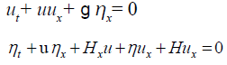
Solving Tsunami equation using the MOL: Consider the instance of the run-up of 2D long wave's occurrence upon a uniform inclining shoreline associated with a vast sea of uniform profundity (Figure 1). The traditional nonlinear shallow-water conditions are [6]:

Figure 1. The one-dimensional problem of Tsunami run-up on a shore.
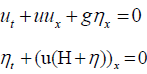 (1)
(1)
where as shown in Figure 1.
u(x, t): is tsunami velocity; η(x, t): is surface elevation (wave amplitude)
H(x) is the variable sea depth; g: is the acceleration due to gravity g=9.8m/s2
x: is the horizontal distance;
t: is the time;
The initial conditions can be written as
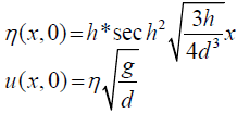 (2)
(2)
Where, h: is an initial wave height; d: is the sea depth in the open ocean.
The exact solutions occur only when H(x) = d they are:
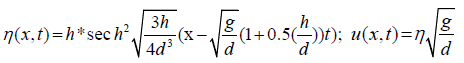 (3)
(3)
The system (1) has no exact solution when H(x) is variable. So, we will solve this system for three different function of H(x) in the form H(x) = ax + 300 which H(x) = 0.5x + 300, H(x) = x + 300 and H(x) = 2x + 300 to show the effect of the slop (a) on the run-up heights and the velocity of tsunami wave.
Tsunamis stages are: the first is formation, the second is midocean propagation, and last is breaking and run-up on the beach.
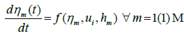
Let x, t be the independent variables and u1, u2, u3, … … . un, η1, η2, η3, …. ηm be the dependent variables associated with a system of PDEs. The general form of a system of PDEs having 1st order time derivatives and 1st order space derivatives may be written as follows:
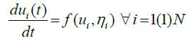 (4)
(4)
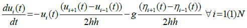
 (5)
(5)
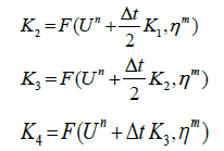
Each ODE of the systems (4, 5), along with current values of the dependent variables as the initial conditions, may be solved by using any of the standard methods to compute the values of the dependent variables. We utilize the classical 4th order Runge- Kutta method. Equations (4, 5) can be rewritten as:
 (6)
(6)
 (7)
(7)
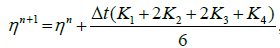
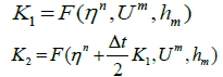
Thus, we have the system of differential equations of one independent variable t. This system can be easily solved by using fourth order Runge–Kutta scheme.
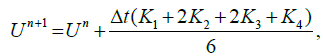 (8)
(8)
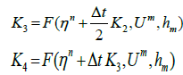
Where, 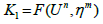
 (9)
(9)
Where,
As done before we have solved Equation (8) using MOLI then we present a comparison between the MOLI results with the exact solution when H(x) = d as shown in Figure 2. It seems that the absolute errors are small at t = 0.5 and increase with increasing the time as shown in Figures 3 and 4.

Figure 2. Comparison of MOLI (dotted line) and exact (solid line) solutions at N =1600, h=2, H(x)=d=20 and t=0, 0.5, 2 and 4.

Figure 3. The absolute error (AE) between the exact solution and the MOLI solution for tsunami equation at what constants at t=0.5, 2 and 4.

Figure 4. Graph of velocity u at shore slope 2.
Analysis of Tsunami equation using the MOL: Tsunami waves were generated with different wave height and depth at different period. It can be observed that an increase in slope causes adecrease in wave height and when the wave height increase the wave length decrease as shown in Figures 5-14. We not that the period didn’t change the properties of the Tsunami wave. Figures 12-14 implies that as the depth of the water decrease the velocity of tsunami increase so in the deep ocean Tsunami have very small amplitude (wave height) and the wave height increase as the depth decrease. Figures 15-20 implies that for a constant height (H(x) = d) when the depth increases the velocity decrease and the elevation become constant.

Figure 5. Graph of elevation η at shore slope 2.

Figure 6. Graph of elevation η at shore slope 1.

Figure 7. Graph of velocity u at shore slope 0.5.

Figure 8. Graph of elevation η at shore slope 0.5.

Figure 9. Graph of velocity u at various H(x) and t=1.

Figure 10. Graph of elevation ηat various sea depths and t =1.

Figure 11. Graph of velocity u at various sea depths at t =1.5.

Figure 12. Graph of elevation η at various sea depths at t =1.5.

Figure 13. Graph of velocity u at shore slope 2 and various values of sea depth in open ocean at t =1.5.

Figure 14. Graph of velocity u at shore slope 2 and various values of sea depth in open ocean at t =1.5.

Figure 15. Graph of elevation η at shore slope 2 and various values of sea depth in open ocean at t =1.5.

Figure 16. Graph of velocity u at various values of sea depth in open ocean at h=2 and t=1.5.

Figure 17. Graph of elevation η at various values of sea depth in open ocean at h =2 and t =1.5.

Figure 18. Graph of elevation η at various values of sea depth in open ocean at h=2 and t=0.

Figure 19. Comparison of MOLI (dotted line) and exact (solid line) solutions of Eq.(1) at N=1600, h=2, d=20 and t =2, 4 and 6 solutions for u.

Figure 20. Comparison of MOLI (dotted line) and exact (solid line) solutions of Eq. (1) at N=1600, h=2, d=20 and t =2, 4 and 6 solutions for η.
Solution of Tsunami equation using HWM
Haar wavelet method: The Haar wavelet is are a symmetrical capacity of exchanged rectangular waveforms where amplitudes can be unique in relation to one capacity to another and de?ned over the interim [0,1] as pursues:
 (10)
(10)
Where 
The integer m = 2j where j = 0, 1, 2, …, J, denote the wavelet level, and k = 0, 1, 2, …, m - 1 is denote the translation parameter. Resolution level known as the integer J. The index i is established according to the formula i = m + k +1. In case of the values m = 1, k = 0. We own i = 2; The value of in is μ = 2M = 2J + 1. Assume we define the collocation points  , with l = 1, 2, …, 2M and the Haar function hi(x). The Haar coefficient matrix is known as HAAR(i, l) = hi(xl) which is a square matrix 2M × 2M.
Method of solution: We can assume that H, L2 [0, 1) is a Hilbert space with the inner product defined by  Since V is a finite-dimensional subspace of H, it is closed and convex. Thus, for w ε H, there are a unique approximation out of V such as g
 (11)
(11)
 (12)
(12)
where the Haar wavelet method coefficients are given by 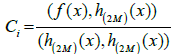 such that (.,.) denotes the inner product, where μ = 2M = 2j+1, C and h(x) are 1 × 2M matrices given by:
 (13)
(13)
Multiplication of Haar wavelet method: It is important to assess the product of  that is called the product matrix of Haar wavelet method. Let
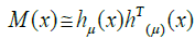 (14)
(14)
where M(x) is 2M × 2M matrix. Multiplying the matrix M(x) by vector C we obtain
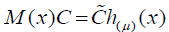 (15)
(15)
where  matrix and called the coefficient matrix. Let R is 2M × 2M matrix. Multiplying the matrix R by vector h(μ)(x) and multiplying the matrix h(μ)(x) by the resulted matrix R h(μ)(x) we obtain
 (16)
(16)
where  matrix and called the coefficient matrix with the powerful properties of Eq. (16) We can achieve
  by away like
  we can convert the Volterra part of integral and Integro-Differential Equations System equations to an algebraic equation.
HWM applied to the Tsunami run-up model yields an analytical solution in terms of rapidly convergent easily computable terms.
Equation (1) written as:
 (17)
(17)
We define the linear operator
We consider the application of the HWM to the model of tsunami Run-up on the coast with the initial conditions. Where the initial wave height (h) and the constant value of sea depth (d) are given by h = 2 and d = 20. And we consider three different cases of shore slopes with the depth function H(x) given by
Case I: Shore slope = 0.5, H(x) = 0.5x + 300
Case II: Shore slope = 1, H(x) = x + 300
Case III: Shore slope = 2, H(x) = 2x + 300
For the Tsunami model we have computed analytic solutions to equation (15) using Maple 15 (Tables 1A-1H).
| x | MOL | HWM |
|---|---|---|
| 0 | 0.775435705843 | 0.7754895431117 |
| 15 | 0.927626747086 | 0.9278187550637 |
| 30 | 1.064755315418 | 1.0647366440529 |
| 60 | 0.361910033228 | 0.361897456040 |
| 75 | 0.138698696189 | 0.138739288119 |
| 90 | 0.049090131969 | 0.049112586589 |
| 105 | 0.016875068044 | 0.016884077653 |
| 120 | 0.005735339986 | 0.005738636481 |
| 135 | 0.001939263041 | 0.001940430796 |
| 150 | 0.000653791689 | 0.0006541999083 |
Table 1A. The values of velocity u at shore slope 2, d=10 and h=2 at t=0.5.
| x | MOL | HWM |
|---|---|---|
| 0 | 0.024695547836 | 0.0245922643554 |
| 15 | 3.726959266545 | 3.7285142696089 |
| 30 | 5.843373800096 | 5.8435239641855 |
| 45 | 4.617805767048 | 4.6162585617936 |
| 75 | 0.914469655265 | 0.9147581475193 |
| 90 | 0.33533007619 | 0.3354912710164 |
| 105 | 0.11910092844 | 0.1191671460289 |
| 120 | 0.04173323531 | 0.0417580771231 |
| 135 | 0.01452155544 | 0.0145305745015 |
| 165 | 0.00173613581 | 0.0017372827749 |
Table 1B. The values of elevation η at shore slope 2, d=10 and h=2 at t=0.5.
| x | MOL | HWM |
|---|---|---|
| 0 | 0.0146767645 | 0.0146561 |
| 15 | 0.0295304605 | 0.0295489 |
| 30 | 0.0695353242 | 0.06953156 |
| 45 | 0.1582343262 | 0.15823748 |
| 60 | 0.3297004405 | 0.3297049 |
| 75 | 0.58442395994 | 0.58442849 |
| 90 | 0.79737141212 | 0.79737165 |
| 105 | 0.74439222240 | 0.74643916 |
| 120 | 0.459331720102 | 0.41615933 |
| 135 | 0.217011889604 | 0.21701489 |
| 150 | 0.091314130163 | 0.0913489 |
Table 1C. The values of velocity u at shore slope 2, d=10 and h=2 at t=1.5.
| x | MOL | HWM |
|---|---|---|
| 0 | -0.42024584 | -0.4208156232 |
| 15 | -0.28024021 | -0.2808516240 |
| 30 | -0.00319321 | -0.0038516193 |
| 45 | 0.600639997 | 0.600684563 |
| 60 | 1.800691310 | 1.800965691 |
| 75 | 3.667549880 | 3.667541649 |
| 90 | 5.378742395 | 5.378715423 |
| 105 | 5.256640812 | 5.25664084 |
| 120 | 3.354546155 | 3.35454566 |
| 135 | 1.630955322 | 1.63095856 |
| 150 | 0.704718125 | 0.704714815 |
| 165 | 0.290193924 | 0.29019392 |
| 180 | 0.116892752 | 0.11689275 |
| 195 | 0.046519873 | 0.04658955 |
| 210 | 0.018365262 | 0.01836562 |
Table 1D. The values of elevation η at shore slope 2, d=10 and h=2 at t=1.5.
| x | MOL | HWM |
|---|---|---|
| 0 | 1.22269209769 | 1.222708384879 |
| 15 | 1.226318884710 | 1.226331637389 |
| 30 | 1.163123922891 | 1.163127093566 |
| 45 | 1.0399381742546 | 1.03993184859 |
| 60 | 0.8761100530607 | 0.87609944751 |
| 75 | 0.6984085017272 | 0.69839912176 |
| 90 | 0.5310853501003 | 0.53107967707 |
| 105 | 0.3889804809915 | 0.38897825424 |
| 120 | 0.2769674718309 | 0.276967397910 |
| 135 | 0.1932186907370 | 0.193219595725 |
| 150 | 0.1328632088968 | 0.132864370631 |
| 165 | 0.090451826012 | 0.090452901556 |
| 180 | 0.061158023987 | 0.0611588959021 |
| 195 | 0.041158981836 | 0.0411596409561 |
| 210 | 0.027612428004 | 0.0276129062761 |
Table 1E. The values of velocity u at shore slope 0.5, d=20 and h=2 at t=0.5.
| x | MOL | HWM |
|---|---|---|
| 0 | 1.4124775362 | 1.4124936789 |
| 15 | 2.3416193724 | 2.3416204856 |
| 30 | 3.0069417436 | 3.0069163387 |
| 45 | 3.2648281925 | 3.2647767328 |
| 60 | 3.1256293454 | 3.1255710977 |
| 75 | 2.71598934708 | 2.7159458972 |
| 90 | 2.19289876937 | 2.1928784260 |
| 105 | 1.67726333464 | 1.6772618619 |
| 120 | 1.23401098686 | 1.2340199796 |
| 135 | 0.88345785062 | 0.8834704292 |
| 150 | 0.62064377369 | 0.6206560071 |
| 165 | 0.43038827925 | 0.4303985338 |
| 180 | 0.29581699704 | 0.2958249364 |
| 195 | 0.20209333266 | 0.2020991967 |
| 210 | 0.13749195049 | 0.1374961563 |
Table 1F. The value of elevation η at shore slope 0.5, d=20 and h=2 at t=0.5.
| x | MOL | HWM |
|---|---|---|
| 0 | 0.4985818076 | 0.4985836857323 |
| 15 | 0.5336565233 | 0.5336615432408 |
| 30 | 0.5996877272 | 0.5997006075876 |
| 45 | 0.6827276484 | 0.6827487558092 |
| 60 | 0.7618775671 | 0.7619008384469 |
| 75 | 0.8131028471 | 0.8131169847658 |
| 90 | 0.8166623672 | 0.8166577866131 |
| 105 | 0.7657027201 | 0.7656801563363 |
| 120 | 0.6699689574 | 0.6699396773769 |
| 135 | 0.5505504249 | 0.5505265903356 |
| 150 | 0.4294116742 | 0.4293984317104 |
| 165 | 0.3216311753 | 0.3216271428251 |
| 180 | 0.2337983357 | 0.2337998131882 |
| 195 | 0.1663473317 | 0.1663511371678 |
| 210 | 0.1165867115 | 0.1165909342995 |
Table 1G. The values of velocity u at shore slope 0.5, d=20 and h=2 at t=1.5.
| x | MOL | HWM |
|---|---|---|
| 0 | 0.34470688975 | 0.34470362511 |
| 15 | 1.24270022801 | 1.24275101653 |
| 30 | 2.15149435851 | 2.15160099089 |
| 45 | 3.02918112501 | 3.02933470122 |
| 60 | 3.79244305608 | 3.79260565183 |
| 75 | 4.327893886213 | 4.32799903195 |
| 90 | 4.533622004821 | 4.53361205666 |
| 105 | 4.373915609464 | 4.37379323263 |
| 120 | 3.908168808445 | 3.90800089538 |
| 135 | 3.265244937672 | 3.26510596417 |
| 150 | 2.582656116358 | 2.58257922024 |
| 165 | 1.958599972169 | 1.95857829096 |
| 180 | 1.440121789292 | 1.44013349656 |
| 195 | 1.035770710691 | 1.03579653611 |
| 210 | 0.733481265177 | 0.73350945764 |
Table 1H. The values of elevation η at shore slope 0.5, d=20 and h=2 at t=1.5.
Discussion and Conclusion
The MOL and HWM for approximating arrangements of Non- Linear Tsunami Model of Coupled Partial Differential Equations. The outcomes announced here give additional proof of the convenience of MOL. The MOL was unmistakably extremely effective and ground-breaking strategy in finding the arrangements of the proposed coupled nonlinear conditions. It is significant that to expand the exactness of the HWM the precision of the arrangement. This prompt increments the many-sided quality of computations. Be that as it may, the MOL is steady, easy to execute and requires moderately little computational assets. The numerical technique created in this investigation to anticipate the run-up of tallness waves gives a basic yet sensibly great forecast of different parts of the run-up process. The outcomes concur well with the exploratory information [9]. From this investigation we see that the technique for lines (MOL) is an appropriate strategy for the examination of long wave marvels started in the shallow water area. Besides, correlations with standard HWM arrangements uncover that the MOL gives a compelling calculation to mimicking shallow water conditions [10-15].
Acknowledgements
The authors are grateful to the anonymous referee for his suggestions, which have greatly improved the presentation of the paper.
References
- Hayashi Y, Munemoto K, Imamura F. Effect of the Emperor seamounts on trans-oceanic propagation of the 2006 Kuril Island earthquake Tsunami. Geophys Res Lett. 2008;35:611-22.
- Koshimura, Imamura F, Shuto N. Characteristics of Tsunamis propagating over oceanic ridges. Journal of Physics. 2001;24:213-29.
- Kowalik. Basic Relations between Tsunami calculation and their physics. Science of Tsunami Hazards. 2003;21:154-73.
- Kowalik Z, Knight W, Logan T, et al. Numerical modelling of the Indian Ocean tsunami. Science of Tsunami Hazards. 2007;17:97-122.
- Kowalik Z, Knight W, Logan T, et al. Numerical modelling of the global tsunami. Science of Tsunami Hazards. 2005;23:40- 56.
- Marchuk AG, Anisimov AA. A method for numerical modeling of Tsunami run-up on the coast of an arbitrary profile. International Tsunami Symposium. 2001;7:7-27.
- Peregrine DH, Williams SM. Swash overtopping a truncated plane beach. J Fluid Mech. 2001;440:391-99.
- Jacobson T. Vorticity on a Barred Beach. J Fluid Mech. 2001;449(1):313-39.
- Gedik N, Irtem E, Kabdasli S. Laboratory investigation on Tsunami run-up. J Ocean Eng. 2005;32:513–28.
- Ramadan MA, Ali MR. An ef?cient hybrid method for solving fredholm integral equations using triangular functions. New Trends in Mathematical Sciences. 2017;5(1):213-24.
- Sadat RE, Ali MR. Application of the method of lines for solving the KdV-Burger equation. Journal of Abstract and Computational Mathematics. 2017;2(2):39-51.
- Ramadan MA, Ali MR. Application of Bernoulli wavelet method for numerical solution of fuzzy linear Volterra-Fredholm integral equations. Communication in Mathematical Modeling and Applications. 2017;2(3):40-9.
- Ali MR. Approximate solutions for fuzzy Volterra integro-differential equations. Journal of Abstract and Computational Mathematics. 2018;3(2):11-22.
- Sadat R, Kassem M. Explicit solutions for the (2+ 1)-dimensional Jaulent–Miodek equation using the integrating factors method in an unbounded domain. Math Comput Appl. 2018;23(1):1-9.
- Ramadan MA, Ali MR. Solution of integral and Integro-Differential equations system using Hybrid orthonormal Bernstein and block-pulse functions. Journal of Abstract and Computational Mathematics. 2017;2(1):35-48.