Research Article - Biomedical Research (2016) Computational Life Sciences and Smarter Technological Advancement
Statistical texture feature set based classification of histopathological images of stomach adenocarcinoma
Anishiya P* and Sasikala M
Department of Electronics and Communication, Guindy, Anna University, Tamil Nadu, India
Accepted date: April 3, 2016
Abstract
Inspection of the biopsy samples microscopically plays a vital role in the definitive diagnosis of cancer. To overcome the subjectivity in pathologists’ decision, objective analysis of the stomach biopsy samples is carried out in this work. At the tissue level, malignancy leads to distortions in glandular structure and nearby supporting tissue namely, stroma. These pathological alterations are known to cause larger variations in the image’s texture. So the proposed method extracts textural features from the histopathological image and classifies them using the SVM classifier. Gray-Tone spatial Dependence Matrix (GSDM), Gray-Level Run Length Matrix (GLRLM), Wavelet transform were used for the extraction of statistical texture features from Region of Interest (ROI). Embedded model of feature selection was carried out. Minimum Redundancy Maximum Relevance (MRMR) scheme was used for Feature ranking. The composite feature set comprising of both the spatial domain (GSDM, GLRLM) and Wavelet domain features showed better discriminating characteristics for the four different classes, (Normal, Well Differentiated, Moderately Differentiated, Poorly Differentiated) achieving a highest classification accuracy of 93.75%.
Keywords
Adenocarcinoma, Biopsy, Texture, Statistical feature set, Support vector machine.
Introduction
Almost 90-95% of the stomach (Gastric) cancer is of epithelial in origin. They are called as Adenocarcinoma of stomach. The internal lining of the stomach consists of glands that are responsible for the secretion of digestive enzyme. These glands are made of epithelial cells which secretes the enzyme into the glandular duct. Malignant tumours arising from these epithelial cells are known as Adenocarcinoma Although the latest advances in the imaging technologies have made non-invasive cancer diagnosis a reality, the confirmatory diagnosis is still done based on the visual examination of the biopsy samples. Biopsies are obtained through the endoscopic examination of the patient. The adenocarcinoma samples are classified as welldifferentiated (Grade I), Moderately-differentiated (Grade II), and Poorly- differentiated (Grade III). Diagnosis and grading are the crucial steps that determine the correct choice of treatment offered to the patients to prolong their survival. Currently it is performed through the visual examination by pathologist. Their judgment is highly subjected to inter and intra observer variations [1]. It consumes a lot of time too.
In order to overcome these drawbacks, the process of automating the histopathological examination of gastric adenocarcinoma images was carried out. This has also paved the way for quantitative assessment of biopsies.
Several studies for the classification and grading of cancer in histopathological tissue samples specific to various organs were found in the literature. In a broad sense these works were mainly oriented towards gland and/or nuclei segmentation [2], and subsequent feature extraction and classification. In some works a sub image which was taken as the representative of the whole image was subjected to feature extraction [3]. In some other works a single image was split into different sub-images and the features from these images were combined in to a single set to characterize the entire image [4]. The feature set comprised of either one of the following features Morphological features, Fractal features [5-8], Topological features, Intensity Based features, Texture [9] or a combination of two or more were used for classification. [10]. The critical step in extracting the cells’ morphological features is its segmentation. Interactive interface, Snakes, was used for the segmentation of the cells obtained through Fine-Needle Aspiration Procedure (FNAP) for breast cancer detection. Fuzzy-C-Means clustering was used for the segmentation of the urinary bladder cells. Exploring the architectural details of the tissue forms the basis of extracting the topological features from the image. This is often performed by constructing a graph on various constituents of the tissue. Voronoi diagram, Delaunay triangulation and minimum spanning tree were the techniques used for graph construction. The features from the graph express the spatial relationship existing between them [11-14]. This work was done on the microscopic images of the adenocarcinoma images. The ROI (Region of Interest) was selected by the pathologist. Colour normalization was carried out in the lαβ colour space using a linear transformation. The features were extracted using GSDM, GLRLM and Wavelet transform. Extracted features were ranked based on the MRMR frame work. SVM classifier was used for feature selection and classification.
Materials and Methods
Data set
A set of 80 images obtained from hospital was used for experimentation. The set consists of 20 Normal images, 19 well differentiated images, 21 moderately-differentiated images, 20 poorly-differentiated images. ROI selection was done by pathologist. The size of the original image is 2048 × 1536. Size of ROI is 512 × 512.
The block diagram of the proposed work is shown in Figure. 1

Figure 1. Block diagram of the computer aided diagnosis system.
Colour normalization
Colour normalization was carried out to compensate for the colour variations. Colour variations due to differences in the quality of the H&E stain and variations in the staining quantity as it was done manually. The colour variations are evident in the Figures 2 and 3. An efficient method for inflicting the colour appearance of a one image (target) on to the other (sample) as proposed in [15] was used. The algorithm is as follows

Figure 2. Sample images used for experimentation. (a). Normal (b). Well-Differentiated. (C). Moderately- Differentiated (d). Poorly- Differentiated.

Figure 3. Colour normalized images. (a). Normal (b). Welldifferentiated (c). Moderately-differentiated (d). Poorlydifferentiated.
(1) Convert the image from RGB colour space to device independent XYZ colour space.
(2) Convert the image from XYZ to LMS colour space.
(3) Convert the details in LMS to logarithmic space.
(4) De-correlate the axes using Principal Component Analysis (PCA)
(5) Obtain the lαβ colour space.
(6) Apply the linear transformation as given in Equation (1).
Convert the data in lαβ colour space to RGB colour space.
The colour transformation was accomplished by matching the statistics namely, mean and standard deviation of the sample image to that of the target image in the lαβ colour space. Well stained image is shown in Figure 2a was fixed as the target image. The over/under- stained images is given in Figures 2b-2d was used as the sample image.
The transformation function is given in Equation (1)
 (1)
(1)
Where l, l? are the mean and standard deviation of the Corresponding images.
Texture feature extraction
As the histopathological visual examination by pathologists mainly depends on the distribution of cellular (nucleus and cytoplasm) components with respect to extra cellular (Lumen, stroma and its nucleus) components, texture analysis is one of the best way to discriminate the adenocarcinoma images.
The following methods were implemented to extract textural information.
Gray-level spatial dependence matrix (GSDM)
It is also called Gray-Level Co-occurrence Matrix (GLCM). It may be viewed as a 2-D accumulator used for storing the frequency count of pixel with gray value i co-occurring with pixel of gray value ‘j’ in a specific linear relationship spatially. As this matrix captures the relationship between a pair of pixels that is, two different pixels, it is used for the extraction of second order statistics (textural features) present in the image. It is a square matrix containing as many number of rows/column as the number of gray levels present in the image. Each element of the matrix C(a, b, Δi, Δj) corresponds to the number of co-occurrence of the pixel a with that of pixel b in the given neighbour-hood separated by a distance of (Δi, Δj) in the specified direction θ, where Δi is called row offset and Δj is called column offset . For practical application θ values were quantized in four particular directions (0?, 45?, 90?, 135?) in correspondence to the pixel under consideration in the digital image. So it is often used for the extraction of directional information present in the image. After the construction of the GSDM matrix, 4 different Haralick features [16] were extracted for discriminating the images based on the textural information present in them. They are given below:
Contrast: It is a measure of intensity difference between a pixel and its neighbour-hood computed over the entire image. It is also called sum of squares variance. Higher the contrast, coarser the texture is.
Whereas finer texture has low contrast value
 (2)
(2)
Correlation: It is a measure of the dependency relationship existing between a pixel and its neighbour over the whole image.
 (3)
(3)
Where μa, μb are the means and σa, are the standard deviations of (a) and (b) respectively.
Energy: It is a measure of the amount of regularity present in the image. It can also be termed as angular second moment.
 (4)
(4)
Homogeneity: It is a measure of degree of proximity of the elements in the GSDM to its diagonal elements. In other words it determines how the pixel intensities are distributed in relation to the homogenous region in the image.
 (5)
(5)
Wavelet transform
Statistics of a sub image (local features) in comparison to the entire image (global features) varies to a large extent. This is mainly due to the heterogeneity of information present in the image. This kind of heterogeneity is mainly constituted by the morphological variation of different objects present in it. For example analysing smaller objects at higher resolution and larger objects at lower resolution gives more information specific to the objects than analysing it on a single scale. The method of analysing an image at various scales is called Multi- Resolution Analysis (MRA). For digital images the MRA is carried out using Discrete Wavelet Transform (DWT). It is based on the concept of sub band coding. Here the resolution of the image is changed through filtering operations and change of scale is obtained through the sub-sampling (up sampling and down sampling) operations. In this method a signal f (i), is sent in to half band low pass filter, d[i] and a half band high pass filter, g [i] simultaneously. The corresponding output is as follows
 (6)
(6)
 (7)
(7)
Both the filter outputs are then down sampled by a factor of 2.Thereby a single level of decomposition is represented as follows
 (8)
(8)
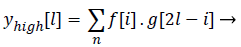 (9)
(9)
Where ylow[l]called Detail coefficients and yhigh[l] are called
Approximation coefficients: Each level of decomposition removes half the number of samples, thereby reducing time resolution by half and doubling the frequency resolution. The most critical factor that influences the efficiency of the extracted feature’s power in discriminating the classes is the type of the wavelet used. The choice of wavelet is purely application specific. The main feature of cancerous histopathological image is abrupt changes in the tissue components. As Daubechies (Db) wavelet can efficiently captures these variations, they were used in this work. Daubechies wavelet of order 2 was used. Energy values extracted from various detail coefficients namely the horizontal, vertical, diagonal details were used as the features for classification. Energy of detail co-efficient for 1-D decomposition is calculated as
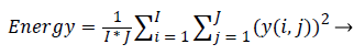 (10)
(10)
= 1, 2 … I, where i= row size; j=1, 2 … J, where j=column size
Gray-level run length matrix (GLRLM)
It is a matrix used for the extraction of the higher order (spatial relation between more than two pixels) statistical features in the image. Here run refers to the set of pixels with the same intensity lying consecutively and collinearly in a given direction. Run length number corresponds to the number of pixels constituting each run. It is calculated by counting the number of times the corresponding run occurs in the image. The matrix can be represented as (u, v, |θ). It means that pixels with gray value of ‘u’ occurs collinearly ‘v’ times adjacent to each other in the direction θ. The features Short Run Emphasis (SRE), Long Run Emphasis (LRE), Gray-Level Non- Uniformity (GLNU), Run Length Non-Uniformity (RLNU), Run Percentage (RPC) introduced by Galloway [17] , Low Gray- Level Run Emphasis (LGRE), High Gray-Level Run Emphasis (HGRE) introduced by Chu et al. [18], Short Run Low Gray-Level Emphasis (SRLGE), Short Run High Gray- Level Emphasis (SRHGE), Long Run Low Gray-Level Emphasis (LRLGE), Long Run High Gray-Level Emphasis (LRHGE) introduced by Dasarathy and Holder [19] were studied.
Feature selection
The irrelevant and redundant features in the feature set adversely affect the classifier’s performance. Also the large number of features tends to over-fit a learning model leading to decreased classifier’s performance, increased computational complexity and storage space. To overcome these problems, feature selection was performed. Embedded model based feature selection was carried out in this work. Informative theoretic approach was used for feature ranking. In particular Minimum Redundancy- Maximum Relevance (MRMR) structure was used for formulating the amount of conditional mutual information that is present in the given set of features. It is then globally optimized through spectral relaxation Features are then arranged in the decreasing order of their weights. Those features with higher weights are given higher ranks. The subsets of features, starting from higher ranks are fed into the classifier. Commencing from the highest ranked feature, the feature set is incremented by one at a time subsequently, while feeding it to the SVM classifier. The subset of the features yielding the highest accuracy was selected as the reduced feature set. 10-fold Cross validation was used as the error estimation technique.
Results and Discussion
A set of 80 images comprising of 20 Normal images, 19 well differentiated images, 21 moderately-differentiated images, and 20 poorly-differentiated images were investigated. ROI selection was done by pathologist. Colour compensation was carried out in the lαβ colour space. GSDM, GLRLM and wavelet features were extracted. MRMR framework was used for feature ranking. SVM classifier was used for feature ranking and classification.
Haralick texture features
In this work, the efficiency of the features contrast, correlation,
Energy, Homogeneity in discriminating the different classes was studied through experimentation. The three important factors that affect the efficiency of the above said features are 1. No. of quantization Levels. 2. Orientation. 3. Distance.
Factor 1. No. of quantization Levels (Q): There exists a trade-off between noise present in the image and textural information while deciding the value of Q. Q was fixed at 32, a level which is sufficient enough to retain the textural information, reduce the noise and computational cost. Uniform Quantization was implemented.
Factor 2. Orientation: The GSDM was constructed for 4 different orientations namely 0º, 45º, 90º, 135º. Table 1 shows the efficiency of the direction specific features in differentiating the 4 different classes for 4 different distances. Table 4 shows the efficiency of direction insensitive features. Mean values were obtained by averaging the feature values of the 4 different orientations. The Mean-Range values set comprise of the features that are in-variant under rotation.
| Distance | 0? | 45? | 90? | 135? | Mean (%) |
|---|---|---|---|---|---|
| 1 | 72.5 | 80 | 72.5 | 71.25 | 73.75 |
| 2 | 67.5 | 78.75 | 73.75 | 75 | 66.25 |
| 3 | 67.5 | 68.75 | 75 | 76.25 | 71.25 |
| 4 | 76.25 | 66.25 | 75 | 83.75 | 75 |
Table 1. Performance of rotation variant features of GSDM for distance 1, 2, 3, and 4 individually.
Factor 3. Distance: It is one of the most important parameter that determines the efficacy of the GSDM features. [20] Suggests the use of range of distances rather than using a single distance for better classification accuracy. As the normal glands are of fine textures, poorly- differentiated class are of coarse textures and the other two classes are intermediary, a distance value of 1 to 4 was chosen for better representation of all the 4 different classes. In order to analyse the effect of using range of distances, features belonging to different distances are grouped together yielding 6 different sets corresponding to the orientations 0?, 45?, 90?, 135?, mean values and the Mean- Range values. Prior to feeding them to the classifier they were subjected to feature selection. This was done to weed out the irrelevant features which can increase the feature space complexity leading to decreased efficiency of the classifier.
A classifier’s performance depends on the separbility of patterns in the given feature space. To find the optimal feature space with highest pattern repeatability, every time while combining two different best feature sets, they were subjected to feature selection. The index value of the GSDM features at 0° orientation is given in Table 2. The impact of feature selection is evident from the Tables 3 and 4.
| Feature Set | Index | Selected Features |
|---|---|---|
| 0? | 1, 2, 3, 4 | Contrast, Correlation , Energy, Homogeneity (Distance-1) |
| 5, 6, 7, 8 | Contrast, Correlation , Energy, Homogeneity (Distance-2) | |
| 9, 10, 11, 12 | Contrast, Correlation , Energy, Homogeneity (Distance-3) | |
| 13, 14, 15, 16 | Contrast, Correlation , Energy, Homogeneity (Distance-4) |
Table 2. Index value of the haralick feature set.
| Accuracy (%) | ||||
|---|---|---|---|---|
| Feature Set | Before feature selection | After feature selection | No.of selected features | Selected features |
| 0? | 72.5 | 85 | 8 | 16, 12, 3, 7, 8, 4, 15, 11 |
| 45? | 71.25 | 85 | 8 | 15, 11, 8, 16, 12, 3, 7, 4 |
| 90? | 76.25 | 85 | 6 | 16, 8, 3, 12, 4, 7 |
| 135? | 76.25 | 83.75 | 8 | 15, 3, 7, 11, 16, 8, 12, 4 |
Table 3. Performance of rotation variant features for combination of distance 1, 2, 3, and 4.
| Accuracy (%) | ||||
|---|---|---|---|---|
| Feature Set | Before feature selection | After feature selection | No.of selected features | Selected features |
| Mean values | 75 | 85 | 8 | 15, 16, 8, 12, 3, 11, 7, 4 |
| Mean-Range | 71.25 | 88.75 | 20 | 12, 31, 4, 8, 16, 28, 24, 32, 15, 1 |
| values | 19, 27 ,20, 23, 3, 11, 7, 6, 9, 17 | |||
Table 4. Performance of rotation in-variant features for combination of distance 1, 2, 3, and 4.
It is interesting to note that the selected features comprises only the features energy and Homogeneity and are devoid of the features contrast and Homogeneity except for the Mean-Range values set . This is in agreement with the work done in [21]. Thus the energy and Homogeneity features capture the variations present among the images of 4 different classes efficiently than the contrast and correlation measures. Similar kind of indexing was adopted for the features from other orientations (45?, 90?, 135?) and for mean values also. The mean value spans the index of 1-16 and the range values span the index of 17-32 in the Mean-Range values category following the same order as given in Table 2.
Table 3 and 4 shows that rather than using a single distance value, combination of different distances has led to increased classifier’s performance. Further the experimentation was done by pooling all the selected features in the Table 3 for the orientations 0?, 45?, 90?, 135?. This is done to improve the classifier’s performance by taking advantage of the increased performance, provided by combination of different distances and different orientations [22]. This pooling of the best features of different orientations has led to an increase in the classifier’s performance to 90%. From Table 5, it is observed that rotation variant features performed better in comparison to the rotation invariant features for a combination of distances 1, 2, 3 and 4.
| Feature Set | Accuracy (%) | No.of selected features |
|---|---|---|
| Rotation variant (0?, 45?, 90?, 135?) |
90 | 18 |
| Rotation In-Variant | 88.75 | 14 |
Table 5. Performance comparison of GSDM rotation-variant and rotation-invariant features for a combination of distances 1, 2, 3, and 4.
GLRLM features
The GLRLM features were also analysed for four different orientations constituting the rotation-Variant set (Table 6). Their mean and range values formed the rotation-Invariant set. As shown in the Table 8, here again the rotation variant features performed better in comparison to their rotation- in variant counter parts. The GLRLM features performed better compared to the Haralick texture features. This is because, Unlike GSDM, the GLRLM gives the spatial relationship between more than two pixels present in the image [23]. Such a measure captures the component specific connectivity information (This information varies depending on the extent of glandular distortions caused by cancerous cell clumsiness, spread, decrease in the cytoplasmic content, lumen deviations, etc.) present in the image.
| Index | Features |
|---|---|
| 1 | SRE |
| 2 | LRE |
| 3 | LGRE |
| 4 | HGRE |
| 5 | SRLGE |
| 6 | SRHGE |
| 7 | LRLGE |
| 8 | LRHGE |
| 9 | RPCD |
| 10 | GLNU |
| 11 | RLNU |
Table 6. Index value of the GLRLM feature set for 0?.
Similar kind of indexing was adopted for the features from other orientations (45?, 90?, 135?) and for mean values also. The mean value spans the index of 1-11 and the range values span the index of 12-22 in the Mean-Range values category following the same order as given in Table 7. The rotation variant set formed out of the selected features in the Table 8, corresponding to the orientations 0?, 45?, 90?, 135? was then subjected to feature ranking and final subset selection. Result of the final composite subset yielding the best accuracy is given in Table 9.
| Feature Set | Accuracy (%) | No. of selected features |
|---|---|---|
| 0? | 78.75 | 3, 7, 4, 8, 5, 9, 6 |
| 45? | 87.5 | 8, 3, 4, 5, 7, 9, 11, 6, 2, 1 |
| 90? | 86.25 | 3, 5, 8, 7, 9, 4, 11, 1 |
| 135? | 82.5 | 3, 8, 5, 9, 4, 1, 11 |
| Mean values | 78.75 | All features |
| Mean-Range values | 83.75 | 20, 1, 22, 15, 3, 16, 6, 21, 17, 18, 9, 14 |
Table 7. Performance of GLRLM features.
| Feature Set | Accuracy (%) | No.of selected features |
|---|---|---|
| Rotation variant (0?, 45?, 90?, 135?) |
91.5 | 11 |
| Rotation In-Variant | 83.75 | 12 |
Table 8. Performance comparison of GLRLM rotation-variant and rotation-invariant features.
| Feature Set | Accuracy (%) | No.of selected features |
|---|---|---|
| Haralick+GLRLM | 93 | 9 |
| Haralick+Wavelet | 90 | 10 |
| GLRLM+Wavelet | 92.5 | 7 |
| Haralick+GLRLM+Wavelet | 93.75 | 13 |
Table 9. Performance comparison of composite feature set.
Wavelet features
Multiresolution analysis of images in the wavelet domain was performed using Haar wavelet. It is best at characterizing the sharp transitions in gray-levels. The glandular distortion produces apical transitions in the gray level. So Daubechies-2 wavelet was used for extracting the class specific information present in the image. 4 Level of decomposition was performed [24]. Energy values extracted from the 3 high frequency components in each sub-band forms the wavelet feature set. As 4 Level of decomposition was performed, 4 × 3=12 features were extracted from the wavelet domain. These 12 features yielded an accuracy of 85% after subjecting them to feature selection, in which case no reduction in the number of features was observed.
Composite features
Table 9 shows the classifier’s performance for combination of different feature sets. The composite feature set was formed by taking only the features that yielded the highest classification accuracy in their respective category. They are then subjected to feature ranking and subsequent optimal subset selection. It is observed that the final sub-set comprising of both the spatial and wavelet domain features yielded the highest classification.
Conclusion
Computer aided Diagnosis and grading system of the stomach adenocarcinoma histopathological digital images is proposed in this work. Haralick features, Wavelet and GLRLM features were first extracted. Embedded based feature selection was carried out using the MRMR scheme and SVM classifier. 10- fold cross validation was used to estimate the performance of the classifier. The effect of 2 important factors namely distance and Orientation, on the extracted Haralick texture features were studied. The results showed that rotation variant features performed better in comparison to the rotation-invariant features. The same scenario was noticed for GLRLM features also. Also the combination of 4 different distances yielded higher accuracy rather than using a single distance for Haralick features. Results show that the composite feature set comprising of the spatial domain and wavelet domain features yielded the highest accuracy of 93.75% surpassing the performance of the individual feature sets.
Acknowledgement
Our sincere thanks to Dr. Jegannathan, Pathologist, KMC, Chennai for his valuable suggestion and supervision in guiding our work. Also thanks to the Health and Family Welfare Department, Tamilnadu for providing us the permission for accessing the images from MMC, Chennai.
References
- Hachung Y, Antoine M, Robert B, Elisabeth L, Jacques D, Stanislas C. Inter-observer agreement on histological diagnosis of colorectal polyps: the APACC study. Gastroenterol Clin Biol 2002; 26: 220-224.
- Christos S, Spiros Kp, Dimitris G, Panagiota R, Dionisis C. Segmentation and Classification of Histopathology Images for Abetting Diagnosis in Urinary Bladder Cancer, 4th International Conference on Experiments/Process/System Modelling/Simulation/Optimization 2011.
- James D, Neil HA, Peter HB, Fiac, Rodolfo M, Frcpath, Peter WH. The Use of Morphological Characteristics and Texture Analysis in the Identification of Tissue Composition in Prostatic Neoplasia. Hum Pathol 2004; 35: 1121-1131.
- Abdelrahim NE, Raouf N, Naguib G, Bayan SS, Mark KB, Alan M. Microscopic image analysis for quantitative measurement and feature identification of normal and cancerous colonic mucosa, IEEE transactions on information technology. Biomedicine 1998; 2: 3.
- Po-Whei H, Cheng HL. Automatic Classification for Pathological Prostate Images Based on fractal analysis, IEEE transactions on medical imaging 2009; 28: 7.
- Stephen G, Rainer HW, Jim M, Peter SH. Lacunarity Analysis: A Promising Method for the Automated Assessment of Melanocytic Naevi and Melanoma 2009.
- Ravi KS, Venkata SP, Jianying ZH, Sergio DC, Wei Q. Comparative study of feature measures for histopathological images of the lung, imaging and applied optics congress in Tucson, Arizona 2010.
- Qureshi H, Rajpoot, Nasir M, Nattkemper T Hans V. A robust adaptive wavelet-based method for classification of meningioma histology images, workshop on optical tissue image analysis in microscopy, histology, and endoscopy (OPTIMHisE), London 2009; 31-42.
- Globocan. IARC Stomach Cancer-Estimated Incidence, Mortality and Prevalence Worldwide 2012
- Stephen G, Rainer HW, Jim M, Peter SH. Lacunarity Analysis: A Promising Method for the Automated Assessment of Melanocytic Naevi and Melanoma 2009.
- Stephen JK, James D, Glenn W, Hoshang B, Deborah T, Peter HB, Peter WH. An automated machine vision system for the histological grading of cervical intraepithelial neoplasia. J Pathol 2000; 192: 351-362.
- Afik BT, Cigdem GD. Graph run-length matrices for histopathological image segmentation, IEEE Transactions on medical imaging 2011; 30: 3.
- Dogan A, Celal C, Cenk S, Cigdem GD, Colour graphs for automated cancer diagnosis and grading, IEEE Transactions on biomedical engineering 2010; 57: 3.
- Nick W, William H, Wolberg OLM. Nuclear feature extraction for breast tumor diagnosis. In IS&T/SPIE 1993 International Symposium on Electronic Imaging: Sci Tech 1993; 1905: 861-870.
- Reinhard E, Adhikhmin M, Gooch B, Shirley P. Colour transfer between images, IEEE computer graphics and applications 2001; 21: 34-41.
- Haralick RM, Shanmugam K, Dinstein I. Textural features for image classification, IEEE transactions on systems, man, and cybernetics 1973; 3: 610-621
- Galloway MM. Texture analysis using gray level runs lengths, Computer Graphics and Image Processing 1975; 4: 172-179.
- Chu A, Sehgal CMA, Greenleaf JF. Use of gray value distribution of run lengths for texture analysis, Pattern Recognition Letters 1990; 11: 415-419.
- Belur VD, Edwin B. Holder, Image characterizations based on joint gray level-run length distributions, (1981) Pattern Recognition Letters 1991; 12: 497-502.
- Soh LK, Tsatsoulis C. Texture analysis of SAR sea ice imagery using gray level co-occurrence matrices, IEEE transactions on geoscience and remote sensing 1999; 37: 780-795.
- SaimaRathore, MutawarraHussain, Muhammad AksamIftikhar, Abdul Jalil, Ensemble Classification Of Colon Biopsy Images based on information rich hybrid features, in computers in biology and medicine, Elsevier 2014; 47: 76-92.
- Soh LK, Tsatsoulis C. Texture analysis of SAR sea ice imagery using gray level co-occurrence matrices, IEEE transactions on geoscience and remote sensing 1999; 37: 780-795.
- Dikshit O. Textural classification for ecological research using ATM images. Int. J. Remote Sensing 1996; 17: 887-915.
- Nguyen K, Bredno J, Knowles DA. Using contextual information to classify nuclei in histology images. IEEE 12th International Symposium on Biomedical Imaging (ISBI) 2015; 995-998.