Research Article - Biomedical Research (2016) Volume 27, Issue 4
Selective cell segmentation using semi-automatic graph cut with adaptive distance penalties
Kazeem Oyeyemi Oyebode* and Jules-Raymond TapamoSchool of Engineering, University of KwaZulu-Natal, Durban, South Africa
- *Corresponding Author:
- Kazeem Oyeyemi Oyebode
School of Engineering
University of KwaZulu-Natal
South Africa
Accepted date: March 28, 2016
Abstract
Selective segmentation provides the opportunity to monitor and assess closely the activities of cells within a confined section of a given cell image. Segmentation of cells through traditional graph cut method is well known; however, when a selective segmentation is desired, the task becomes cumbersome. In order to take advantage of the optimum segmentation of graph cut while simultaneously adopting a local (selective) segmentation strategy, a third term is added to the graph cut energy function. The term is referred to as adaptive distance penalties (ADP). ADP constrains graph cut to any selected region of interest while using a reference image to achieve a semi-automatic segmentation. Experiments show that for fairly homogeneous cell images, the proposed model outperforms the grab cut selective segmentation.
Keywords
Graph cut, Graph cut energy function, Selective segmentation, Semi-automatic segmentation.
Introduction
Graph cut segmentation has been widely used because of its ability to segment any given image globally with promising results. In order to deliver a robust segmentation, in [1], the graph cut energy function is fitted with two terms: the data term and the smoothness term (these two terms will be discussed later). In literature, many contributions have been put forward to address various shortfalls of graph cut with encouraging results, for example: in the area of parameter selection in [2] and [3]; the addition of shape priors in [4-6]; and graph cut with compact shape prior in [7]. Furthermore, graph-cut-based active contour is also researched in [8,9], segmentation of dense nuclei is discussed in [10] and the usage of point prior is discussed in [11]. A two-stage graph cut for touching cell segmentation is proposed in [12]. A more recent automatic graph cut segmentation is put forward in [13] and [14], and also, improved cervical cell segmentation in [15]. Lastly, an improved graph cut for lungs segmentation is developed in [16] and a selective segmentation of moving objects in [17]. These modifications to graph cut have been adapted to solve many segmentation problems, while little research has been proposed with respect to selective cell segmentation.
The advantage of the global segmentation strategy of graph cut can also be a setback, as regions which are of no interest, having similar pixels to objects of interest, are captured during segmentation. This development does not provide the opportunity to investigate sections of cell images in isolation. When biologists are interested in analysing a specific section of a cell image, a selective segmentation is necessary. Selective segmentation provides the opportunity to monitor a group of cells in isolation when other parts of the image are occupied by noise or debris. A biologist may also find this selective segmentation fulfilling as it provides the opportunity to concentrate on important areas holding crucial information at a given time. For example, the close monitoring of infected cells by tuberculosis or the interaction of tuberculosis and cells in a particular section of cell image, can be segmented and monitored in isolation.
Furthermore, selective segmentation, which is also described as selective information gathering can be useful when data-gathering is required for a single cell. For example, data such as shape, size and texture of a single cell can be gathered automatically to enhance automated diagnosis. In addition, this method can also be useful in determining whether a cell under investigation has improved or deteriorated over time under the influence of an array of potential drugs, to cure, for example, cancer or tuberculosis.
In this research, a semi-automatic segmentation is put forward within the context of a modified graph cut segmentation. This research is inspired by the selective segmentation put forward in [18]. In [18], a modified graph cut (grab cut) is proposed where the algorithm operates automatically and segmentation results are updated as user redefines or adjusts sample foreground and background pixels. A border matting model is then used to strengthen object edges of the grab cut result. The grab cut tool can be found in Microsoft Office.
The rest of the paper is organised as follows: graph cut segmentation approach is discussed, followed by the introduction of proposed model. In the next section, experiments, discussions and conclusion are put forward in that order.
Graph cut concept
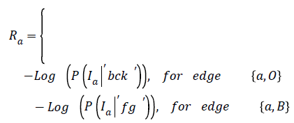
The representation of an image is formulated into a graph structure G = (V, E), where V is the set of pixels in the image context and E is the set of edges between elements of V. Additional nodes O and B are encapsulated in set V and serve as terminal nodes. For a given pixel a, (where a ϵ V), two categories of edge exist with terminal nodes O and B. For instance, for pixel a, the first category gives rise to the edge/ link {a, O} and {a, B} as seen in figure 1. The second gives rise to the edge/link that exists within pixels neighbouring of a, these edges are {a, b} and {a, g} (b, g ϵ V) (see Figure 1). These edges have weights assigned to them; for instance the assignment of weights to edges {a, O} and {a, O} is based on Eq. (1). This equation depends on sample foreground pixels ‘fg’ and sample background pixels ‘bck’. The sample data can be acquired interactively by user marking portions of the foreground and background of image to be segmented. It can also be learnt based on domain knowledge prior to segmentation. The latter approach is investigated in this research.
 → (1)
→ (1)

Figure 1: Image represented as a graph.
In Equation (1), the weight on edge {a, O} is determined based on the negative logarithm of the probability of how pixel intensity fits into an observed data- . In the same line of argument, the weight on terminal link {a, B} is a function of how the negative logarithm of the probability of pixel intensity Ia fits into an observed data-‘fg’.
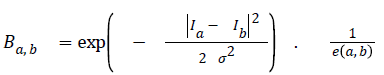
The second term is called the smoothness term- it acts on links holding neighbouring pixels. The smoothness term encourages an arrangement where neighbouring pixels having similar intensity values are encouraged to retain their identities cohesively and dissimilar pixels are discouraged from sharing same colour identity. The equation for giving weights to neighbouring edges for the smoothness term is seen in figure 2.

Figure 2: Selective cell segmentation using graph cut.
 → (2)
→ (2)
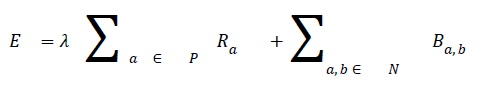
Ia and Ib are intensity values of neighbouring pixels, and σ gives the degree of concern for pixel similarity. These two terms (the data term and the smoothness term) are fitted into the graph cut energy function in Equation (3). regulates the relative relevance of the data term to the smoothness term. -is the Euclidean distance between pixels a and b. Minimising Equation (3) results in an image partitioned into foreground and background.
 → (3)
→ (3)
where P is the total number of pixels in a given image and the set of neighbouring pixels is N.
Method
Adaptive distance penalties (ADP)
In order to segment region of interest, an adaptive distance term is added to graph cut energy function which penalises pixels not included in the region of interest. The modified energy function is shown in Equation (4).
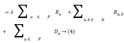
The third term D, which is the adaptive distance penalty (ADP), acts on link {a, O} and {a, B} where a ϵ P. D can be either zero or one. When D is zero for a given pixel, it means it belongs to a region of interest defined by user; however, when D is one for a given pixel, it falls outside the region of interest. For example, assume set P consists of pixels a,b,c,e,f,g where a,c,g are foreground pixels and are background pixels as shown in figure 2(a). figure 2(b) gives the highlighted region indicating region of interest which means the values of D for pixels a,b,f,g is zero, while that of c and e is one. figure 2c shows the graph representation of this scenario and figure 2d gives the final segmentation output when the energy function in Equation (4) is minimised using the algorithm in [19].
Semi-automatic segmentation
Within the context of graph cut segmentation, sample foreground and background pixels can be selected either manually or automatically. Selecting manually yields an interactive segmentation as seen in [1]. Many authors have also leveraged the interactive graph cut segmentation for segmenting nerve cells, for example, in [20]. Sample pixels can also be selected automatically, this development give rise to an automatic graph cut segmentation [21]. However, in this research, we adopt the semi-automatic graph cut segmentation option where a reference image is picked from a given dataset, and foreground and background pixels are already labelled. The idea is to bridge the gap between the time-consuming interactive segmentation and the automatic segmentation. The automatic segmentation may not be a robust approach to segment images from a wide array of datasets, since every dataset has its own uniqueness.
Leveraging the semi-automatic segmentation, a reference image (Figure 3a) is picked from a given dataset and manually segmented as seen in figure 3b. This information in figure 3b serves as a guide to the proposed algorithm to learn about the variability of the foreground and background pixel intensity levels of a given dataset. This process can also be considered as a domain knowledge acquisition process.

Figure 3: (a) Original image; (b) manually segmented image.
Region of interest selection and weight assignment to graph
The proposed model provides an interactive platform where users select region of interest. Figure 7a shows how region of interest is selected. Table 1 gives weight distribution in the graph formulation based on explanation in figure 2. Figure 4 gives an overview of the proposed model.

Figure 4: Overview of proposed model.

Figure 5: (a) Selective segmentation of grab cut; (b) result of selective segmentation of grab cut, with circled cell in (a) absent in (b).

Figure 6: (a) Region of interest selection; (b) ground truth; (c) segmentation by proposed model; (b) grab cut segmentation.

Figure 7: (a) Region on interest selection; (b) ground truth; (c) grab cut segmentation; (d) segmentation by proposed model.
| Edge | Weight | Applied to |
| {a,b} | Ba,b | {a,b} ∈ N |
| {a,0} | ̶ Log (P (Ia |′ bck ′ )) | D=0 |
| 0 | D=1 | |
| {a,B} | infinity | D=1 |
| ̶ Log (P (Ia |′ fg ′ )) | D=0 |
Table 1: Assigning weights to graph edges.
Experiments
Dataset
Experiments are carried out on fluorescence microscopy cell images (U2OS) in [22]. This dataset consists of fairly homogeneous cells and uses 188 cells for the evaluation process.
Evaluation
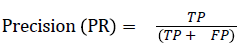
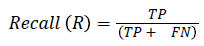
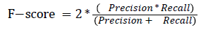
The pixel-based evaluation framework is used to investigate the segmentation accuracy of the proposed model. In doing this, various metrics such as the precision (PR), f-score (Fscore) and recall (R) are used. Equation (5-8) give their formulae. In these equations, true positive (TP) reflects the total number of foreground pixels in a segmented image S that are found to be true foreground pixels in the ground truth T. True negative (TN) reflects the total number of background pixels in S that are found to be true background pixels in T. False positive (FP) is the total number of foreground pixels in S but these foreground pixels are seen as background pixels in T. False negative (FN) is the total number of background pixels in S but these background pixels are seen as foreground pixels in T.
 → (5)
→ (5)
 → (6)
→ (6)
 → (7)
→ (7)
Evaluation and Results
The proposed model is implemented using Matlab 2014, on a Windows 7, core i5 machine. Based on these metrics (PR, R, F-score and RI), proposed model shows improved performance over existing grab cut algorithm. The value of FN shows that proposed model reasonably minimises the shrink bias of graph cut as opposed to grab cut. The value of FN for proposed model is almost doubled in grab cut as seen in table 2. Figure 7 gives the visual segmentation results while figure 6 gives visual results on elongated cells.
| Model | PR (%) | R (%) | F-Score | RI (%) | FN |
| Grab cut | 97.36 | 74 | 83.8 | 97.5 | 31319 |
| Proposed model | 98.0 | 85 | 91 | 98.5 | 18497 |
Table 2: Comparison of proposed model with grab cut.
Discussions
This research explored selective cell segmentation within the context of graph cut. Selective cell segmentation provides an opportunity to carry out cell analysis in isolation. In order to get a better result for selective cell segmentation using semi-automatic graph cut, we used a single image from a given dataset to inform the algorithm about the variability of foreground and background pixels. This shows that custom-made segmentation methods, which are a function of domain knowledge, can outperform generic ones. Figure 5a gives an example to buttress this point. The small white circles shows seed points informing the grab cut algorithm to retain these regions as foreground. However, the portion circled with green is a cell, which is not seen as a foreground cell even after several seed points are inserted as seen in figure 5b. This development also explains the fact that most of the grab cut selective segmentation is heavily interactive as user needs to put seed points on almost every cell to segment them, as seen in figure 5a. This is unlike ours, where selective segmentation is semi-automatic, once knowledge acquisition (foreground and background characteristics are learned by the algorithm) is carried out. It is also worth pointing out that little noise is attributed to results obtained from the proposed model in figures 6c and 7d while this is not the case for grab cut, though this noise can be minimised via morphological processing. One of the downsides of the proposed model is that for every new dataset, the model is trained to learn about the characteristics of foreground and background pixels while valuable time is wasted on manually segmenting cells to achieve this process.
Conclusion
This research introduces the selective cell segmentation using the adaptive distance penalties on semi-automatic graph cut.
There are many benefits of the proposed model (selective segmentation); one of them is the restriction of segmentation to area of interest. The second benefit is the ability to minimise noise since only a section of the image may be important. The third is that the model provides a platform for further research in the area of tracking selected segmented cells. This model is evaluated using fairly homogeneous cell images; it would be interesting to see how it performs on highly heterogeneous cells. This will be our next line of research.
References
- Boykov Y, Jolly M. Interactive Graph Cuts for Optimal Boundary & Region Segmentation of Objects in N-D Images. International Conference on Computer Vision, Vancouer, 2001.
- Peng B, Veksler O. Parameter Selection for Graph Cut Based Image Segmentation. 2008.
- Candemir S , Akgul YS. Adaptive Regularization Parameter for Graph Cut Segmentation. Springer-Verlag 2010; 6111: 117--126.
- Wang H, Zhang H, Ray N. Adaptive shape prior in graph cut image segmentation. Pattern Recognition 2013.
- Lang X, Zhu F, Hao Y, Wu Q. Automatic Image Segmentation Incorporating Shape Priors via Graph Cuts. International Conference on Information and Automation, China 2009.
- Freedman D, Zhang T. Interactive Graph Cut Based Segmentation with shape priors. IEEE Conference on Computer Vision and Pattern Recognition 2005.
- Das P, Veksler O, Zavadsky V, BoyKov Y. Semiautomatic Segmentation with Compact Shape Prior. Image and Vision Computing 2005.
- Chen C, Li H, Zhou X, Wong STC. Constraint Factor Graph Cut–Based Active Contour Method for Automated Cellular Image Segmentation in RNAi Screening. National Institute of Health 2008.
- El-Zehiry NY, Elmaghraby, A. A graph cut based active contour for multiphase image segmentation. 15th IEEE International Conference on Image Processing, San Diego, CA 2008.
- Qi.J. Dense Nuclei Segmentation Based on Graph Cut and Convexity-Concave Analysis. Journal of Microscopy 2014; 253: 42-53.
- Vicente S, Kolmogorov V, Rother, C. Graph cut based image segmentation with connectivity priors. Conference on Computer Vision and Pattern Recongnition 2008.
- Danek O, Matula P, Ortiz-de-Solorzano C, Munoz-Barrutia A, Maska M. Segmentation of Touching Cell Nuclei Using Two Stage Graph Cut Model. Springer-Verlag 2009; 411 -419.
- Dimopoulos S, Mayer CE, Rudolf F, Stelling J. Accurate cell segmentation in microscopy images using membrane patterns. Bioinformatics 2014; 30: 2644-2651.
- Kechichian R, Gong H, Revenu M, Lezoray O, Desvignes M. New data model for graph-cut segmentation:application to automatic melanoma delineation. IEEE International Conference on Image Processing (ICIP) 2014.
- Zang L, Kong H, Chin CT, Wang T, Chenc S. Cytoplasm segmentation on cervical cell images using graph cut-based approach. Biomedical materials and engineering 2014; 24: 1125-1131.
- Oluyide O. Automatic Lung Segmentation using Graph Cut Optimization. Automatic Lung Segmentation using Graph Cut Optimization unpublished Master's dissertation University of KwaZulu-Natal, Durban, South Africa 2015.
- Malcolm J, Rathi Y, Tannenbaum A. Multi-Object Tracking Through Clutter Using Graph Cuts. Workshop on Non-rigid Registration and Tracking through Learning (in ICCV) 2007.
- Rother C, Kolmogorov V, Blake A. "GrabCut": interactive foreground extraction using iterated graph cuts. ACM Transactions on Graphics (TOG) 2004; 23: 309-314.
- Boykov Y, Kolmogorov V. An Experimental Comparism of Min-Cut/Max-Flow Algorithms for Energy Minimization in Vision. IEE Transactions on PAMI 2004; 26: 1124-1137.
- Vu N, Manjunath BS. Graph cut segmentation of neuronal structures from transmission electron micrographs. Proc’s Int. Conf. Image Processing (ICIP), San Diego 2008.
- Chen C, Li H, Zhou, X. Automated segmentation of drosophila RNAi fluorescence cellular images using graph cuts. Lecture Notes in Computer Science 2007; 116-125.
- Coelho LP, Shariff A, Murphy RF. Nuclear segmentationtation in microscope cell images: a hand-segmented dataset and comparison of algorithms. IEEE International Symposium on Biomedical Imaging: From Nano to Macro 2009.