- Biomedical Research (2016) Volume 27, Issue 3
Performance evaluation and comparative analysis of various machine learning techniques for diagnosis of breast cancer.
Kanchanamani M*, Varalakshmi PerumalKarpaga Vinayaga College of Engineering and Technology, Kanchipuram, Tamil Nadu, India
Accepted date: February 17, 2016
Abstract
Breast cancer is heterogeneous and life threatening diseases among women in world wide. The aim of this paper is to analyze and investigate a novel approach based on NSST (Shearlet transform) to diagnosis the digital mammogram images. Shearlet Transform is a multidimensional version of the composite dilation wavelet transform, and is especially designed to address anisotropic and directional information at various scales. Initially, using multi scale directional representation, mammogram images are decomposed into different resolution levels with various directions from 2 to 32. In this work we investigated five machine learning algorithm, namely SVM (Support Vector Machine), Naïve Bayes, KNN LDA and MLP, which are used to categorizes decomposed image as either cancerous (abnormal) or not (normal) and then again abnormal severity is further categorized as either benign images or malignant images. The evaluation of the system is carried out on the MIAS (Mammography Image Analysis Society) database. The tenfold cross-validation test is applied to validate the developed system. The performance of the five algorithms was compared to find the most suitable classifier. At the end of the study, obtained results shows that SVM is an efficient technique compares to other methods.
Keywords
Breast cancer, Benign, Malignant, Statistical features, Shearlet transform, Support vector machine, Naïve Bayes , KNN, LDA, MLP.
Introduction
Breast cancer is considered a major health problem in women. The occurrence of breast cancer is increasing globally. According to the statistical reports World Health Organization (WHO), breast cancer is the top cancer in women both in the developed and the developing world. In 2007, it was reported that 202,964 women in the United States were diagnosed with breast cancer and 40,598 women in the United States died because of breast cancer. A comparison of breast cancer in India with US obtained from Globocon data, shows that the incidence of cancer is 1 in 30. However, the actual number of cases reported in 2008 were comparable; about 1, 82, 000 breast cancer cases in the US and 1, 15, 000 in India. A new global study estimates that by 2030, the number of new cases of breast cancer in India will increase from the current 115,000 to around 200,000 per year.
According to Globocan data (International Agency for Research on Cancer), India is on top of the table with 1.85 million years of healthy life lost due to breast cancer and moreover A recent survey in united kingdom proved that breast cancer is not only a problem of young women but it is also a problem of old age woman those who have crossed the age of sixty or even seventy. Discrete Shearlet Transform based system is approached [1] for Microcalcification classification. The Energy of the sub band is used as a feature and nearest neighbor classifier used for the classification. The K-Nearest Neighbor (KNN) classifier is used in the classification stage. A microcalcification image in the Mammography Image Analysis Society (MIAS) database [2] is taken for evaluation.
The overview of most related and recent method for the development of CAD system [3] is described. The wavelet based model constructed in [4] and 217 mammograms images from mini MIAS is considered for testing purpose. KNN is used for classification and the results were compared with SVM. The Receiver Operating Characteristic (ROC) curve analysis is used as the performance measure. Discrete Shearlet Transform based system is implemented [5] for texture classification. Shearlet s band signature, entropy is used as a feature and nearest neighbor classifier used for the classification. The performance of the work is analyzed using Brodatz texture database.
A CAD method is suggested in [6] for early detection of masse tumor in breast images with the help of the size and shape. Discrete Shearlet Transform based mass classification is discussed in [7]. The GLCM feature energy is extracted from the decomposed images and KNN is used classification purpose. A CAD system illustrated in [8] which extracts firstorder statistics features using Histogram-based approach. DDSM database image is used for evaluation. Noise from the images is removed using morphological techniques called opening-by-reconstruction and closing-by-reconstruction and then images are segmented using Otsu method.
A CAD system using Shearlet transform is adopted in [8] for classification of breast tumors in ultrasound images. The AdaBoost algorithm is used as classifier and the outputs were compared with wavelet and GLCM based methods. Homomorphic Filtering [9] is used to enhance the images and with the help Shearlet transform, ROI image is decomposed and features are extracted. SVM is used as classifier to categorize the mass images. The performance metrics Sensitivity, specificity and accuracy are calculated. The research paper is arranged as follows: Section 2 introduces the methodology used in the system; Shearlet Transform and Support Vector Machine in a concise manner. Section 3 describes the experimental results. Section 4 includes the conclusion.
Materials and Methods
The proposed system for the classification of breast cancer is built using Shearlet Transform and various classifiers. This section describes the theoretical information about Shearlet Transform, SVM, NB, MLP, KNN and LDA.
Shearlet transform
Shearlet transform is a new concept equipped with a rich mathematical structure, and can capture the information in any direction. The Shearlet transform has the following main properties: well localizing, parabolic scaling, and highly directional sensitivity, spatially localizing and optimally sparse.
The Shearlet representation forms a tight frame which decomposes a function into scales and directions, and is optimally sparse [10-13] in representing images with edges. The continuous Shearlet transform for an image f is defined as the mapping
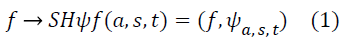
where ψ is a generating function, a> 0 is the scale parameter, S ϵ R is the shear parameter,
t ϵ R2 is the translation parameter, and the analyzing elements ψa,s,t (Shearlet basis functions) are given by
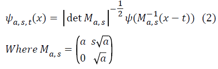
Each element ψ a,s,t has frequency support on a pair of trapezoids at several scales, symmetric with respect to the origin, and oriented along a line of slope s. The Shearlet ψ a,s,t form a collection of well-localized waveforms at various scales a, orientations s and locations t. Image decomposition using Shearlet transform is done two stages namely, decomposition of multi-direction and multi-scale.
1. Multi-direction decomposition of image using shear matrix S0 or S1.
2. Multi-scale decompose of each direction using wavelet packets decomposition.
In step (1), if the image is decomposed only by S0, or by S1, the number of the directions is 2(l+1)+1. If the image is decomposed both by S0 and S1, the number of the directions is 2(l+2)+2. The Image decomposition using Shearlet transform is shown in figure 1 and feature extraction using Shearlet transform [14] is shown in figure 2.

Figure 1. Image decomposition using Shearlet transform.

Figure 2. Feature extraction for two levels Shearlet decomposition with eight directions.
SVM classifier
Support vector machine, SVM [15] is a powerful, robust and sophisticated supervised machine learning approach. It is based on the statistical learning theory. It was firstly proposed by Cortes and Vapnik from his original work on structural risk minimization and then modified by Vapnik. Figures 3 and 4 give the basic principles of SVM. When the data is not linearly separable, the algorithm works by mapping the input space to higher dimensional feature space, through some nonlinear mapping chosen a priori (Figure 1), and constructs a hyper plane, which splits class members from non-members (Figure 2).

Figure 3. Linear SVM hyper plane construction.

Figure 4. SVM topology in hyperspace.
SVM introduces the concept of ‘margin’ on either side of a hyper plane that separates the two classes. Maximizing the margins and thus creating the largest possible distance between the separating hyper plane and the samples on either side, is proven to reduce an upper bound on the expected generalization error.
Naïve bayes classifier
It is one of the frequently used methods for supervised learning. The Naive Bayes is a quick method for creation of statistical predictive models. NB is based on the Bayesian theorem. This classification technique analyses the relationship between each attribute and the class for each instance to derive a conditional probability for the relationships between the attribute values and the class. During training, the probability of each class is computed by counting how many times it occurs in the training dataset.
Multilayer perception classifier
MLP is a feed forward neural network trained using the back propagation algorithm. MLP networks consist of three layers: an input layer, hidden layer is one or more and an output layer. Figure 5 shows MLP feed forward Neural Network.

Figure 5. MLP feed forward neural network.
KNN classifier
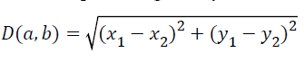
KNN is a method for classifying objects based on closest training examples in the feature space. In KNN, an object is classified by a majority vote of its neighbors, with the object being assigned to the class most common amongst its k nearest neighbors. The nearest neighbor classifier is designed to classify the images. The classification is done by using minimum distance measure. Let us consider a=(x1, y1) and b=(x2, y2) are two points. The Euclidean distance between these two points is given by
Linear discriminant analysis classifier
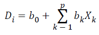
Linear Discriminant Analysis is a one of the Supervised Learning algorithms, which constructs one or more discriminant equations Di (linear combinations of the predictor variables Xk) such that the different groups differ as much as possible on D. It predicts the class of an observation X by the class whose mean vector is closest to X in terms of the discriminant variables. Discriminant function is defined as
Results
MIAS datasets
In this study, Mammographic Image Analysis Society (MIAS) database [2], a benchmark dataset used by most of the researchers is considered for system evaluation. The distribution of different cases available in MIAS database is shown in table 1. There are totally 322 mammogram images of left and right breast acquired from 161 patients.
| Cases | Total images | Benign | Malignant |
|---|---|---|---|
| Normal | 207 | - | - |
| Micro calcification | 25 | 12 | 13 |
| Circumscribed masses | 23 | 19 | 4 |
| Speculated masses | 19 | 11 | 8 |
| Ill-defined masses | 14 | 7 | 7 |
| Architectural distortion | 19 | 9 | 10 |
| Asymmetry lesion | 15 | 6 | 9 |
| Total | 322 | 64 | 51 |
Table 1. MIAS database images.
| S.No | Feature | Expression |
|---|---|---|
| 1 | Mean (or) First Movement | 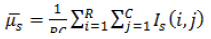 |
| 2 | Variance (or) Second Movement | 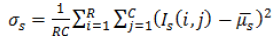 |
| 3 | Skewness (or) Third Movement | 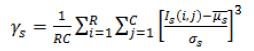 |
| 4 | Kurtosis (or) Fourth Movement | 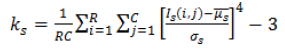 |
| 5 | Contrast | 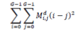 |
| 6 | Correlation | 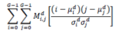 |
| 7 | Energy | 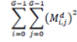 |
| 8 | Homogeneity | 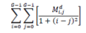 |
| 9 | Entropy | 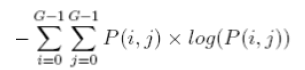 |
| 10 | Sum of Squares | 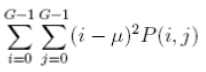 |
| 11 | Sum Average | 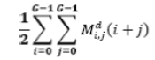 |
| 12 | Sum Entropy | 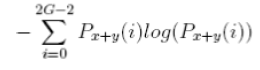 |
| 13 | Difference Entropy | 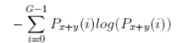 |
| 14 | Cluster Prominence | 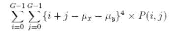 |
| 15 | Sum Variance | 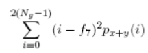 |
| 16 | Difference Variance | 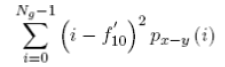 |
| 17 | Maximum Probability |  |
| 18 | Mean Absolute Difference |  |
| 19 | Information measure of Correlation 1 |  |
| 20 | Information measure of Correlation 2 |  |
| 21 | Standard Deviation |  |
Table 2. Extracted features for diagnosis.
All the 64 benign images and 51 malignant images, totally 115 abnormal images are considered for this study irrespective of the type of abnormalities. From the database, 70 normal images are randomly chosen and considered for performance evaluation.
Feature extraction stage
The original mammograms in MIAS are very big size (1024 × 1024 pixels) and almost 50% of the whole image comprised of the background with a lot of noise. Preprocessing is an important issue in low level image processing. Preprocessing [16] stage is required to remove the areas that are not related to the detection region (pectoral muscle and any artifact labels that can be applied on mammogram). Therefore cropping process was performed manually to eliminate the noise and background information and Regions of Interest (ROI) image of size 256 × 256 is cropped from the original image. Figure 6a shows the original mammogram Benign image Mbd005 and Figure 6b shows the corresponding ROI Benign image. Figure 8a shows the original mammogram Malignant Image Mbd271 and Figure 8b shows the corresponding ROI Malignant image.

Figure 6. A-Original benign image Mbd005 (1024 x1024); b-ROI benign image Mbd005 (256 × 256).

Figure 7. Decomposed resultant 5 (4 higher and 1 lower) sub band of ROI Benign Image Mbd005 (256 × 256).

Figure 8. A-Original Malignant Image Mbd271 (1024 ×1024); BROI Malignant Image Mbd271 (256 × 256).
After cropping, Shearlet transform is applied on ROI to decompose the images and then first order statistical features, spatial gray level dependant feature and second order statistical features, totally 21 features have been extracted from the decomposed image. From 21 features [17], 4 features namely Variance, Standard Deviation, Skewness and Kurtosis are selected and used for evaluation purpose. The decomposition level from 2 to 4 with various directions from 2 to 32 is used in this study and the ROI images are transformed into the aforementioned levels and directions. Figures 7 and 9 shows the resultant decomposed ROI images of Benign and Malignant respectively for 2 levels and 2 directions. Figure 10 shows the functional block diagram of the developed diagnosis scheme. The number of sub band is calculated by using the formula.

Figure 9. Decomposed resultant 5 (4 higher and 1 lower) sub band of ROI Malignant Image Mbd271 (256 × 256).

Figure 10. Functional Block Diagram of Proposed diagnosis Scheme.
No.of Sub band=No.of Levels × No.of Directions +1;
Classification stage
In the classification phase, two problems are considered. In first phase the classifiers namely SVM, NB, MLP, KNN, and LDA are trained separately by using normal and abnormal Shearlet moments and in the second phase also the classifiers namely SVM, NB, MLP, KNN, and LDA classifier are trained separately by using benign and malignant Shearlet moments of training mammogram images.
Performance measures
The efficiency of the developed model is evaluated using performance metrics such as TP, FP, TN, FN Sensitivity, specificity, precision, F-measure, error rate and classification accuracy. These performance metrics are evaluated using the confusion matrix. A confusion matrix outputs a number of correctly and incorrectly classified images by an analyzed scheme, which is shown in table 3.
| Actual State | Predicted State | |
|---|---|---|
| Classified as True | Classified as False | |
| Class is True | TP | FN |
| Class is False | FP | TN |
| True Positive (TP)-number of Normal image is correctly classified True Negative (TN)-number of Abnormal image is correctly classified False Positive (FP)-number of Normal image is wrongly classified as Abnormal images False Negative (FN)-number of Abnormal image is wrongly classified as Normal images Sensitivity or Recall or True Positive Rate = TP / (TP+FN) |
||
Table 3. Confusion matrix.
Classification Accuracy=(TP+TN)/(TP+FP+TN+FN)
Precision=TP/(TP+FP), False Positive Rate=FP/(FP+TN)
Specificity=TN/(TN+FP) or (1- False Positive Rate)
F-measure=2*Recall*Precision /Recall+Precision
Error Rate=(FP+FN)/(TP+FP+TN+FN)
Table 4 and Table 5 display accuracy of several of the classifier used in this developed model for normal/abnormal cases and benign/malignant cases respectively.
| SVM | NB | MLP | KNN | LDA | |
|---|---|---|---|---|---|
| Correctly Classified Images | 166 | 124 | 124 | 140 | 140 |
| Incorrectly Classified Images | 24 | 66 | 66 | 50 | 50 |
| Classification Accuracy (%) | 87.3 | 65.2 | 65.2 | 73.6 | 73.6 |
Table 4. Classification Accuracy rate of the various Classifiers for Normal/Abnormal case.
| SVM | NB | MLP | KNN | LDA | |
|---|---|---|---|---|---|
| Correctly ClassifiedImages | 111 | 70 | 58 | 66 | 71 |
| Incorrectly ClassifiedImages | 9 | 50 | 62 | 54 | 49 |
| ClassificationAccuracy (%) | 92.5 | 58.3 | 48.3 | 55.0 | 59.1 |
Table 5. Classification Accuracy rate of the various Classifiers for Benign / Malignant case.
Table 6 and Table 7 exhibit the performance metrics comparison of several of the classifier used in this developed model for normal/abnormal cases and benign/malignant cases respectively. Table 8 shows the error rate of the various classifiers of this approach.
| Classifiers/Observation | TP | FP | TN | FN | Recall or Sensitivity or True Positive Rate (TPR) | Specificity | Precision | False Positive Rate (FPR) | F-score or F-measure | Matthews |
|---|---|---|---|---|---|---|---|---|---|---|
| SVM | 46 | 24 | 120 | 0 | 1 | 0.833 | 0.657 | 0.167 | 0.793 | 0.917 |
| NB | 30 | 50 | 94 | 16 | 0.652 | 0.653 | 0.375 | 0.347 | 0.476 | 0.653 |
| MLP | 23 | 43 | 101 | 23 | 0.5 | 0.702 | 0.349 | 0.298 | 0.41 | 0.601 |
| KNN | 28 | 32 | 112 | 18 | 0.6 | 0.772 | 0.46 | 0.228 | 0.524 | 0.692 |
| LDA | 28 | 32 | 112 | 18 | 0.6 | 0.772 | 0.46 | 0.228 | 0.524 | 0.692 |
Table 6. Performance Comparison of various Machine Learning Algorithms for Normal / Abnormal case.
| Classifiers / Observation | TP | FP | TN | FN | Recall or Sensitivity or True Positive Value | Specificity | Precision | False Positive Value | F-score or F-measure | Matthews |
|---|---|---|---|---|---|---|---|---|---|---|
| SVM | 58 | 2 | 53 | 07 | 0.892 | 0.964 | 0.967 | 0.036 | 0.928 | 0.928 |
| NB | 50 | 35 | 20 | 15 | 0.769 | 0.363 | 0.588 | 0.636 | 0.667 | 0.566 |
| MLP | 29 | 26 | 29 | 36 | 0.446 | 0.527 | 0.527 | 0.473 | 0.483 | 0.487 |
| KNN | 41 | 30 | 25 | 24 | 0.632 | 0.453 | 0.572 | 0.543 | 0.600 | 0.544 |
| LDA | 38 | 22 | 33 | 27 | 0.584 | 0.600 | 0.633 | 0.400 | 0.600 | 0.593 |
Table 7. Performance Comparison of various Machine Learning Algorithms for Benign / Malignant case.
| Error Rate | SVM | NB | MLP | KNN | LDA |
|---|---|---|---|---|---|
| Error Rate for Normal/Abnormal Images | 0.12 | 0.34 | 0.34 | 0.26 | 0.26 |
| Error Rate for Benign/Malignant Images | 0.07 | 0.41 | 0.51 | 0.45 | 0.41 |
Table 8. Comparison of error rate of various Classifiers.
The ROC (receiver operating characteristic) plots of various classifier for benign/malignant cases is illustrated in figure 11a and normal/abnormal cases is explained in figure 11b. Table 9 exhibits the comparison of the proposed work with the already existing systems. Table 9 describes the comparison of the proposed method with other existing approaches for computer aided diagnosis.

Figure 11. A-benign / malignant; B-normal / abnormal.
| Authors & Year | Features Extracted | Classifier Used | Classification Accuracy Obtained (%) |
|---|---|---|---|
| W. Borges Sampaio, et al. [18] | Shape, texture using geostatic function | SVM | 80.0 |
| Wang et al. [19] | Curvilinear, GLCM, Gabor, Multi-resolution statistical features | structured SVM | 91.4 |
| Y.Ireaneus Anna Rejani, et al.[15] | Shape Feature based DWT | SVM Classifier | 88.75 |
| Moayedi F et al 2010 [20] | Contourlet Features | SVM | 82.1 |
| Ioan B. et al. 2011 [21] | Gabor wavelets and directional features | SVM | 84.37 |
| Proposed Method | Shearlet Moments, GLCM, statistical features | SVM | Normal/Abnormal:87.3Benign /Malignant :92.5 |
Table 9. Comparison of proposed system with other existing methods.
Discussion
In this research paper we addressed several machine learning techniques to find a best breast cancer diagnosis model and classification accuracies were compared. The proposed approach is focused on classification of mammogram images as either normal or abnormal (benign or malignant) using various classifiers. The experiments were conducted with MIAS database images. From the results, it is came known that a better classification accuracy 87.3, achieved at level 4 with direction 8 for normal and abnormal classification using SVM classifier and the better classification accuracy 92.5 is achieved at level 3 with direction 8 to distinguish between benign and malignant using SVM classifier [22].
Conclusion
From the experiments analysis, it can be inferred that SVM classifier yields better classification accuracy in both cases when compared with other classifiers results. It is also observed that the classification accuracy of the KNN and LDA are same for normal/abnormal cases and more over it is clear that the classification accuracy of MLP and NB classifiers are same for normal/abnormal cases. Hence this manuscript concludes that SVM classifier is identified as the best method for breast cancer diagnosis compare to other classifiers used in this approach.
References
- Ali AJ, Janet J. Discrete Shearlet Transform Based Classification of Microcalcification in Digital Mammograms. J Comp Appl 2013; 6: 1-3.
- http://peipa.essex.ac.uk/pix/mias/
- Rangayyan RM, Xu J, Elnaqa I, Yang Y. Computer aided detection and diagnosis of breast cancer with mammography recent advances. IEEE Trans InfTechnol Biomed 2009; 13: 236-251.
- Prathibha BN, Sadasivam V. Multi Resolution Texture Analysis of Mammograms Using Nearest Neighbor Classification Techniques. Int J Info Acqui 2010; 7: 109-118.
- Vivek C, Audithan S. Texture classification by Shearlet band signatures. Asian J Sci Res 2014; 7: 94-99.
- Charan BP, Sinha GR. Abnormality Detection and Classification in Computer-Aided Diagnosis (CAD) of Breast Cancer Images. J Med Imaging Health Informa 2014; 4: 881-885.
- Ali A, Janet JJ. Mass Classification in Digital Mammograms Based on Discrete Shearlet Transform. J ComputSci 2013; 9: 726-732.
- El Abbadi NK, Elaf A, Al Taee J, Breast Cancer Diagnosis by CAD. Int J ComputAppl 2014; 100: 975-8887.
- Anusha DS. A Hybrid Scheme for Mass Detection and Classification in Mammogram. Int J EngSci Res Tech 2014; 3: 1591-1593.
- Easley G, Demetrio L, Wang-Q L. Sparse directional image representations using the discrete Shearlet transform. ApplComput Harmon Anal 2008; 25: 25-46.
- Guo K, Labate D. Optimally Sparse Multidimensional Representation Using Shearlets. SIAM J Math Anal 2007; 39: 298-318.
- Guo K, Labate D. Characterization and Analysis of Edges Using the Continuous Shearlet Transform. SIAM J Imaging Sci 2009; 2; 959-986.
- Lim WQ. The discrete Shearlet transform : a new directional transform and compactly supported Shearlet frame. IEEE Trans Image Process 2010; 19: 1166-1180.
- Schwartz WR, da Silva RD, Davi LS, Pedrini H. A Novel Feature Descriptor Based on the Shearlet Transform. 2011 18th IEEE International Conference on Image Processing, Brussels, 1033-1036.
- Rejani YIA, Selvi ST. Early Detection of Breast Cancer using SVM Classifier Technique. Int J ComputSciEng 2009; 1: 127-130.
- Ponraj MN, Jenifer ME, Poongodi P, Manoharan JS. A Survey on the Preprocessing Techniques of Mammogram for the Detection of Breast Cancer. J Emerg Trends ComputInformaSci 2011; 2: 656-664.
- http://www.uio.no/studier/emner/matnat/ifi/INF4300/h08/undervisningsmateriale/glcm.pdf
- Sampaio WB, Diniz EM, Silva AC, de Paiva AC, Gattass M. Detection of masses in mammogram images using CNN, geostatistic functions and SVM. ComputBiol Med 2011; 41: 653-664.
- Wang D, Shi L, Ann Heng P, Automatic detection of breast cancers in mammograms using structured support vector machines, Neurocomputing2009; 72: 3296-3302.
- Moayedi F, Azimifar Z, Boostani R, Katebi S. Contourlet-based mammography mass classification using the SVM family. ComputBiol Med 2010; 40: 373-383.
- Ioan B, Gacsadi A. Directional features for automatic tumor classification of mammogram images. Biomed Signal Process Control 2011; 6: 370-378.
- Huang L, Shi J, Wang R, Zhou S. Shearlet-Based Ultrasound Texture Features for Classification of Breast Tumor. 2013 Seventh International Conference on Internet Computing for Engineering and Science, Shanghai, 116-121.