Research Article - Journal of Psychology and Cognition (2016) Volume 1, Issue 1

Effects of the number of objects and locations on attentional allocation and processing in a visual short-term memory task.

Aymen Ben Abbes¹, Yousri Marzouki^2,3 and Thierry Ripoll²

¹University of Tunis El Manar (Institut Supérieur des Sciences Humaines de Tunis), Tunisia.

²Aix-Marseille Université (Laboratoire de Psychologie Cognitive, CNRS) Marseille, France.

³Qatar University, Doha, Qatar.

*Corresponding Author:

Yousri Marzouki
Laboratoire de Psychologie Cognitive
Aix-Marseille Université, 3 place Victor Hugo
13331 Marseille, France.
Tel: +33 4 13 55 09 73
E-mail: yousri.marzouki@univ-amu.fr

Accepted date: October 07, 2016

Abstract

Using a partial report procedure, we tried to dissociate the effect of increasing the number of attended locations from that of increasing the number of objects (digits) appearing in these locations. Participants had to allocate their attention to different locations among a set of distractors (letters). After a delay of 500 ms they had to process either one, two, three or four digits appearing at one, two, three or four previewed locations. We found that the capacity of attentional allocation over locations decreased at three attended locations and also after the increase in the number of objects while attending to four locations. The same procedure was used in Experiment 2, except that digits were used as distractors to eliminate the possible attentional re-allocation bias towards targets during the processing phase. We introduced in Experiment 3 a color contrast between targets and distractors in order to facilitate their discrimination and to reduce the spatial configuration effect of locations. The results are in line with Experiment 1 findings and showed that the processing of multiple objects is constrained by two interacting difficulties. The first relies on resources distribution over the attended locations whereas the second relies on parallel encoding of objects.

Keywords

Attentional allocation, Division of attention, Capacity threshold.

Introduction

Our visual system is continuously flooded by a huge amount of information, which constantly challenges the way we allocate our attention over space when we simultaneously select and process the most relevant "items". The most popular description in literature of the attentional allocation is the “spotlight” metaphor, which suggests that attention can operate as a beam toward a circumscribed location in order to enhance information processing at this particular position [1,2]. It has been assumed that performance can be significantly damaged when the visual system has to attend to many locations simultaneously due to the cost induced by distributing attention over different locations [3,4]. However, a growing substantial body of data suggests that spatial attention deployment allows the participants to pay attention to non-contiguous locations or objects while they inhibit irrelevant positions or objects interposed between them [5-8]. For example, Awh and Pashler used a partial report technique in which observers had to systematically report the identity of two targets presented at separate locations within a 5-by-5 stimulus matrix [5]. There was a valid condition in which two targets appeared at previously cued locations. In the invalid condition, one of the two targets appeared directly between the cued locations (the medial position). The authors found a strong capacity to attend to the cued locations without selecting the intervening ones. Whatever the conclusions made by these investigations, their main aim was to test the capacity to select targets among distractors and to process these targets simultaneously (detection, identification, memorization, etc.). Accordingly, the performance was contingent upon two sequential difficulties: firstly, the participants had to attend to the critical locations of targets to extract them from distractors, and secondly, they had to encode the properties of targets to enable their full representation. However, even if these two distinctive difficulties had been underlined in some studies [9-11], there was no systematic dissociation between them in the above-mentioned research.

Xu and Chun provided an interesting framework addressing this issue called the neural object-file theory. The latter highlighted the presence of two stages of processing: the object individuation and the object identification. In the first stage objects are individuated and selected from a visual scene and in the second stage objects are encoded and processed by higher visual areas. The authors stated also that this individuation-identification framework requires two distinct stages that are not necessarily separate to guarantee an efficient processing. Most important to our study, Xu and Chun claimed that given the capacity limitation in both individuation and identification processes and in order to process a complex visual scene with multiple objects, visual attention needs to be shifted to different part of the scene [11].

However, in Huang and Pashler, Kraft et al. and Xu and Chun, studies no specific information was provided about the particular difficulties in attentional deployment over many locations, on the one hand, and those related to the multiple processing of targets, on the other [9-11]. Generally, these two sequential difficulties (or costs) have been mapped together without considering performance fluctuation when i) the number of attended spatial locations increases and ii) the subsequent increase of perceptual load under the effect of an increasing number of objects. Stated differently, the attentional distribution over many positions in space in order to optimize the selection of one object is different from the situation in which we must split our attention into many locations in order to process all objects appearing in these locations. In the latter case, there is an initial difficulty of dividing attention over locations and a subsequent one linked to the multiple encoding of objects.

In the present work, we sought to empirically dissociate these two types of difficulties. To do so, we used a partial report paradigm, largely inspired by Awh and Pashler study, by which we manipulated separately the number of locations and the number of objects [5]. Our aim was twofold: i) to determine the cost generated by increasing the number of locations on which depends the attentional selective allocation capacity, and ii) to determine the cost resulting from the increase in the number of objects, which is related to processing capacity. The selective cost was assessed by comparing reporting performance when allocating attention to one, two, three or four locations, apart from the number of objects that could appear in them. The processing cost was estimated by contrasting the reporting performance with one, two, three or four objects.

In our task, observers previewed an array of distractors and had to allocate their attention to specific empty spots in the array corresponding to locations in which targets were most likely to appear. The number of these empty locations varied from one to four. This same array disappeared and reappeared with digits (targets) that occupied the previously empty locations. The number of these digits also varied from one to four, and observers had to report the identity of one of them. Making predictions based on these separate manipulations of number of locations and objects could be difficult, because no systematic variation of these factors had been done in previous research. However, one may expect additive effects of both factors, in which case a linear decrease in performance would be observed as the number of attended locations and the number of processed targets increase. We could also predict that each increase in the number of locations could lead to a loss in performance, which would be emphasized as the number of objects increases. For example, when we moved from two to three locations or from three to four locations, we could expect a decrease in performance due essentially to the growing difficulty in maintaining attention at these locations. Moreover, with a fixed number of locations (two, three or four), increasing the number of objects that could appear in them could be accompanied by a supplementary loss of performance. In the second case, we could expect a linear decrease in performance only as the number of locations decreases or only as the number of objects increases. Performance could be basically contingent upon the difficulty in maintaining attention over many locations and less sensitive to the increase in the number of objects. Conversely, it could be slightly dependent on the number of attended locations but much sensitive to the increase in the number of objects. A final possible prediction could be the possible effect of the number of objects when a certain number of attended locations is reached. In such a case, we would observe a non-linear decrease in performance because of an interaction of the two factors.

Experiment 1

Method

Participants: Ten students from Aix-Marseille University participated in the experiment. All reported having normal or corrected-to-normal vision without visual or neurological problems.

Stimuli and design: The experiment was displayed on a 14-inch computer screen and was controlled using E-Prime 2.0 software® [12]. The participants were tested individually in a dimly lit room. They were seated at a viewing distance of about 70 cm from the computer screen. The number of locations (1, 2, 3 and 4) was crossed with the number of objects (1, 2, 3 and 4) in a within-subjects design as shown in Table 1. 1 location/1 object (1L/1O), 2 locations/1 object (2L/1O), 2 locations/2 objects (2L/2O), 3 locations/1 object (3L/1O), 3 locations/2 objects (3L/2O), 3 locations/3 objects (3L/3O), 4 locations/1 object (4L/1O), 4 locations/2 objects (4L/2O), 4 locations/3 objects (4L/3O), and 4 locations/4 objects (4L/4O). Note the unbalanced structure of the design. This manipulation provided accurate information about the relative cost of each factor. Such cost was considered very low when the participants were confronted with 1 location/1 object and very high when they had to attend to 4 locations/4 objects.

Table 1. The non-orthogonal structure of the experimental design.

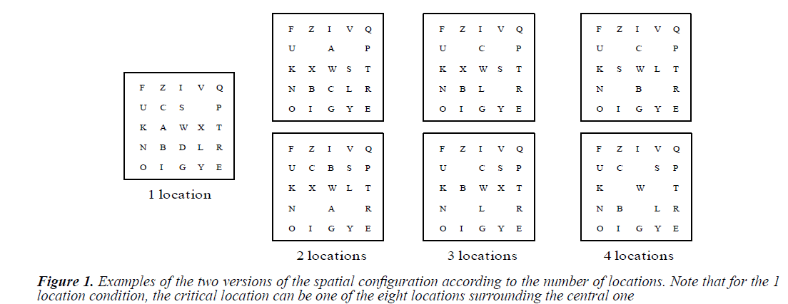
All stimuli were presented within a centrally placed 5 × 5 array of evenly spaced positions. Each stimulus subtends approximately 6.36° on each side from the central fixation. Letters and digits appearing within these locations were approximately 1.27 cm tall and 1.02 cm wide. The visual angle for stimuli appearing within the central 3 × 3 portion of the array was estimated at 3.2°. Apart from the one location condition in which the digit appeared at one of the eight positions surrounding the central positions, two different spatial configurations were used for each location condition (Figure 1).

During all trials, the stimulus array contained 21 uppercase letters and 1, 2, 3 or 4 digits. This set of letters (from the 26 letters of the alphabet) and digits (from 1 to 9) was randomly sampled without replacement. All stimuli were presented as black objects against a white background.

Procedure

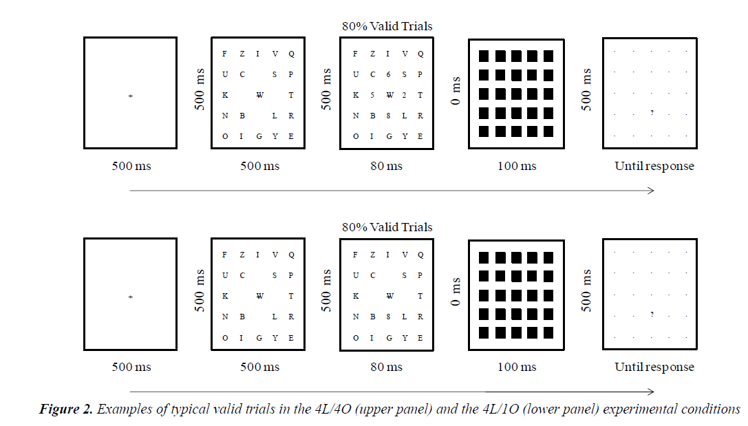
Prior to the experiment, the participants performed a practice session containing 24 trials; this was followed by 600 experimental trials presented randomly. At the beginning of each trial, a fixation point was presented at the center of the screen (Figure 2). The participants were instructed to focus their gaze on this fixation during the trial. Each trial began by pressing the space-bar button. After an interval of 500 ms, the distractors appeared for 500 ms and the participants were instructed to focus their attention on the empty locations presented in this array, because they were more likely to be occupied by targets. These locations always appeared within the central 3 × 3 portion of the 5 × 5 array. This manipulation aimed to equilibrate lateral masking for each of the nine critical locations (and so targets). Five hundred milliseconds after the offset of this array, the critical array containing distractors and targets appeared for 80 ms. This exposure time was sufficient to prevent eye movements or attentional switching between targets. A total of 480 valid trials (80%) and 120 invalid trials (20%) were randomized during the experiment. The 480 valid trials were evenly divided by ten experimental conditions (48 trials/condition). The same goes with 120 invalid trials (12 trials/condition). In the invalid conditions, digits did not appear in the previewed empty locations 20% of the time and only appear at adjacent or distant locations from the previewed ones within the 3 × 3 array matrix. On invalid trials, the locations of targets varied according to experimental conditions. In the 1L/1O condition, the target appeared adjacent to the previously empty location or distant from it. In the 2L/1O and 2L/2O conditions, the target (s) appeared directly between the two previously empty locations (adjacent position condition) or distant from them. In the 3L/1O, 3L/2O, 3L/3O, 4L/1O, 4L/2O, 4L/3O and 4L/4O conditions, the target (s) only appeared adjacent to the previously empty locations; the absence of a distant position condition was due to the specific spatial configuration wherein three or four locations were used, which did not allow locating targets at positions contiguous to previously empty locations. Immediately after the offset of the critical array, a masking array (composed of 25 black squares) occluded the entire 5 × 5 grid for 100 ms. Finally, after 500 ms, the masking array was replaced by a 5 × 5 grid of dots and a post-cue question mark that indicated where one of the targets had appeared. The post-cue also ensured that the participants were accurately informed of target location even during invalid trials. At this level, the participants made an “unspeeded” report of the identity of the target digit by pressing one of the keyboard numeric pad buttons from 1 to 9. After this, a new trial began.

Figure 1. Examples of the two versions of the spatial configuration according to the number of locations. Note that for the 1 location condition, the critical location can be one of the eight locations surrounding the central one.

Table 2. Percent of correct responses as a function of the number of locations, the number of objects and experimental conditions in Experiment 1 (Mean ± standard errors).

Results

The percentage of correct responses was calculated for each condition. Table 2 reports the mean accuracies.

Given the non-orthogonality of the design and the withinsubjects procedure used in this experiment with different participants, it was necessary to explicitly take into account the possible random effects of participants on the accuracy of the data. Thus, we performed a multilevel regression analysis on the accuracy of the data using the linear mixed-effect (LME) model technique [13-15], which is currently becoming the standard technique to analyze this type of data [16,17]. This enabled us to consider fixed and random effects simultaneously in greater detail than possible with traditional by item/by participant averaging. Moreover, the LME technique allowed us to robustly test simple effects and interactions from an unbalanced design.

Mean accuracies were calculated as a function of number of locations, number of objects, and validity. The LME analysis revealed significant main effects of number of locations, [t (5816)=-7.75, p<0.0001] (Whereas denotes the degrees of freedom calculated under the multi-level model's assumptions were confirmed using a Markov Chain Monte Carlo sampling approach [13]), number of objects, [t (5816)=-3.28, p<0.0005], and validity [t (5816)=-6.99, p<0.0001]. We observed a significant interaction between number of locations and number of objects, [t (5816)=2.98, p<0.005]. There was also a significant interaction between number of locations and validity [t (5816)=6.09, p<0.0001] and between number of objects and validity [t (5816)=2.76, p<0.01]. The triple interaction between the three factors was significant [t (5816)=-2.98, p<0.01].

We further investigated the possible presence of mixed effects (i.e., random slopes) between number of locations and participants and between number of objects and participants. We did not find any evidence for significant individual differences across participants in the magnitude of the effects of number of locations or number of objects (ps>0.1). Hence, there was no reason to consider individual results separately, instead of the whole group of participants.

Figure 2. Examples of typical valid trials in the 4L/4O (upper panel) and the 4L/1O (lower panel) experimental conditions.

Effects of the Number of Locations and the Number of Objects in the Valid Condition

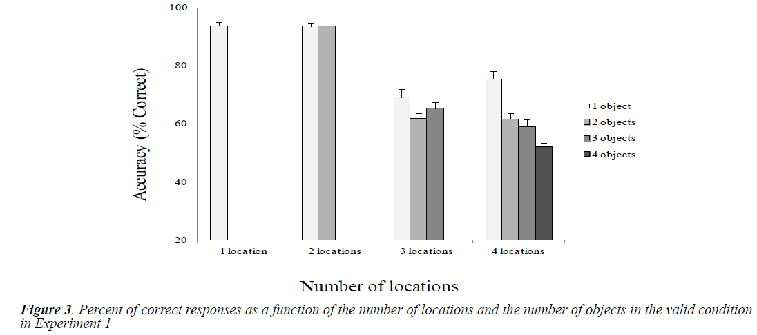
Figure 3 shows the mean accuracies as a function of the number of locations and objects in the valid condition.

We examined differences between conditions related to the number of locations and the number of objects by performing paired t comparisons. Table 3 shows the results. Globally, we observed a significant decline in performance in conditions of three and four locations compared with that in conditions of one and two locations. Surprisingly, with one object, performance was higher in the four-location condition than in the three-location condition. Regarding the effect of number of objects, there was a linear decrease in performance only in the four-location condition.

The very significant performance drop in 3-location condition is not linear. When moving from two to three locations, the performance seemed to cross an important threshold in terms of difficulty to allocate the divided attention but not in terms of processing difficulty. Whereas from three to four locations, we cannot say that the difficulty of attentional allocation has increased (no difference for the 3-location condition for 1, 2 and 3 objects.

Table 3. Paired t comparisons between experimental conditions in the valid condition in Experiment 1.

Effects of the Number of Locations and the Number of Objects in the Invalid Condition

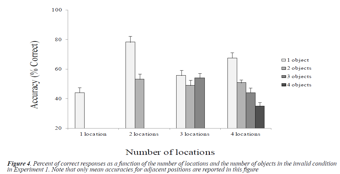
Figure 4 shows the mean accuracies as a function of the number of locations and objects in the invalid condition.

We analyzed differences between the conditions related to the number of locations and the number of objects by performing paired t tests. Table 4 presents the results. The most noticeable effect was the low accuracy in the one-location condition, particularly compared with the two-location condition (with one object). Moreover, we observed a linear decrease in performance as the number of objects increased in the two-location and four-location conditions, but we observed no such effect in the threelocation condition. We found that the targets presented at adjacent invalid positions were better reported than those presented at distant invalid positions, except for the 1L/1O condition, in which no significant difference was observed: adjacent position (1L/1O) vs. distant position (1L/1O), t (9)=0.76, p=0.46; adjacent position (2L/1O) vs. distant position (2L/1O), t (9)=2.24, p=0.05; adjacent position (2L/2O) vs. distant position (2L/2O), t (9)=4.63, p<0.005.

Figure 3. Percent of correct responses as a function of the number of locations and the number of objects in the valid condition in Experiment 1.

Table 4. Paired t comparisons between experimental conditions in the invalid condition in Experiment 1.

Figure 4. Percent of correct responses as a function of the number of locations and the number of objects in the invalid condition in Experiment 1. Note that only mean accuracies for adjacent positions are reported in this figure

Discussion

The results from Experiment 1 clearly showed dissociation between the impact of the number of locations on the selection and the number of objects on the processing. Hence, the appearance of digit targets in the attended locations allowed them to be processed as a different category relative to the letter stimuli used as distractors making the attention to be re-allocated toward them. Such hypothesis can be supported by the demonstrated targetflanker congruity effect according to which there is a reduced flanker (i.e., distractor) effect when distractors were semantically different from targets [18-22]. Thus, we cannot rule out the possibility that the processing operation involved in Experiment 1 may be facilitated by a kind of object-based attentional allocation that occurred during the targets display.

Experiment 2

Experiment 2 aimed to eliminate the possible attentional re-allocation bias towards targets during the processing phase. Therefore, we used the same experimental manipulation as in Experiment 1 except that digits were used as distractors instead of letters. In doing so, we sought to limit the attentional allocation process to the duration of locations' display. Consequently, the manipulation of objects would exclusively reflect the cost linked to their multiple processing since no facilitation based upon an extra-location effect would be allowed during objects processing.

We have showed in Experiment 1 that the attentional reallocation towards targets enhanced the amount of resources attributed to their locations, whereas no such possibility can occur in Experiment 2. Moreover, the sizable validity effect across all conditions in Experiment 1 can be attributed to the contrast category effect (digits vs. letters) especially when targets appeared in invalid locations. The latter entailed more attentional attraction to their locations and an increase in the capacity to process them. On the contrary, distractors and targets in Experiment 2 belong to the same category (all digits) which could weaken such advantage.

We therefore expect a very low performance with respect to the processing of objects in invalid conditions. We also expect a larger difference in favor of 4-location condition relative to 3-location condition.

Participants

Ten students from Aix-Marseille University participated in Experiment 2. All reported having normal or correctedto- normal vision without visual or neurological problems.

Stimuli and Design

The design is the same as in Experiment 1 except that targets and distracters were all digits.

Procedure

The procedure was exactly the same as in Experiment 1.

Results

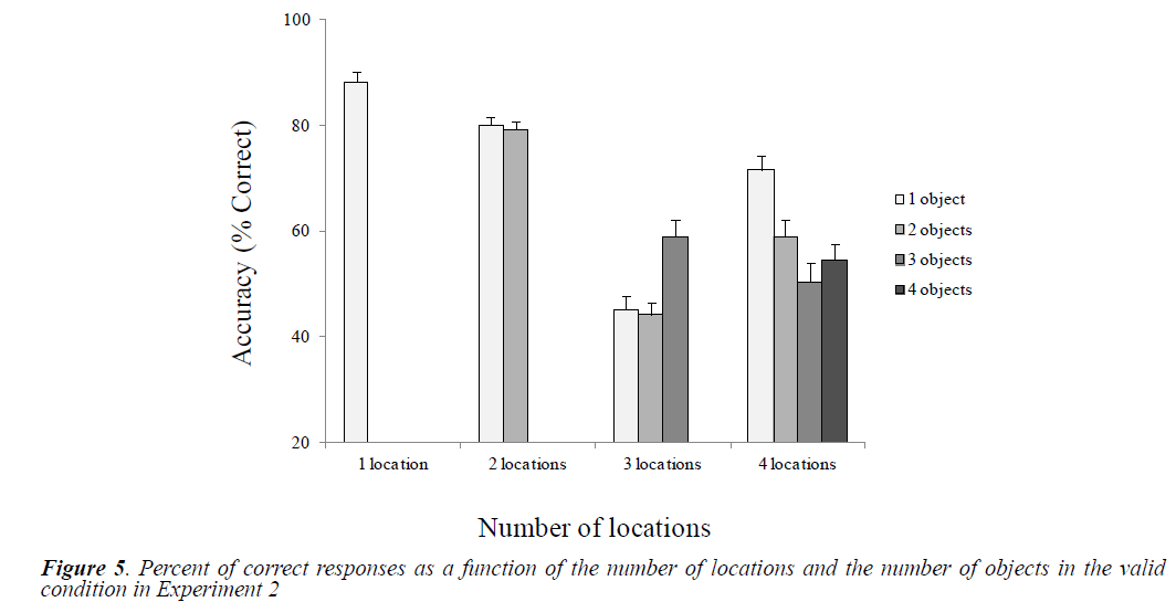
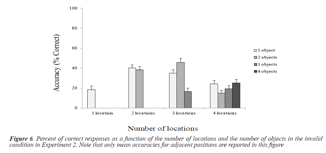
Mean accuracies were reported as a function of the number of locations and objects in the valid and invalid conditions (Figures 5 and 6).

The LME analysis was conducted as a function of the number of locations, the number of objects, and validity. The results showed significant main effects of the number of locations, t (5816)=-6.54, p<0.0001, the number of objects, t (5816)=-3.98, p<0.0001, and validity, t (5816)=- 5.89, p<0.0001. We also found significant interactions between the number of locations and the number of objects, t (5816)=3.90, p<0.0001, between the number of locations and validity, t (5816)=3.98, p<0.0001, and between the number of objects and validity, t (5816)=2.14, p<0.05. The triple interaction between the three factors was also significant, t (5816)=-2.36, p<0.05.

However, the LME analysis did not show the presence of mixed effects (i.e., random slopes) or significant individual differences across participants on the magnitude of the effects of the Number of locations, or the Number of objects, p_s>0.1. Consequently, the whole group of participants was considered for the analysis. The following analysis focused on the differences between conditions related to the number of locations and objects in valid vs. invalid conditions.

Figure 5.Percent of correct responses as a function of the number of locations and the number of objects in the valid condition in Experiment 2.

Figure 6.Percent of correct responses as a function of the number of locations and the number of objects in the invalid condition in Experiment 2. Note that only mean accuracies for adjacent positions are reported in this figure.

Effects of the Number of Locations and the Number of Objects in the Valid Condition

We performed paired t-test comparisons to examine differences between conditions related to the number of locations and the number of object (Table 5). Globally, we observed a significant performance drop in the conditions of 3 and 4 locations compared to the conditions of 1 and 2 locations. When a single or two objects had to be processed, the performance was higher in the 4-location condition than in the 3-location condition. Regarding the effect of Number of objects, we found a significant linear decay in performance only in the 4-location condition as the number of objects increases.

Table 5. Paired t comparisons between experimental conditions in the valid condition in Experiment 2

Effects of the Number of Locations and the Number of Objects in the Invalid Condition

Overall, the accuracy was very low in invalid conditions (e.g. less than 15% in 4L/2O). Paired t-test comparisons were conducted to analyze differences between conditions related to the number of locations and the number of objects (Table 6). The most interesting effect was the low performance obtained in the 1-location condition compared to the other conditions with only one object. Similarly, the performance was lower with 4 locations compared to conditions with 2 or 3 locations (but not with three objects). Furthermore, we observed a performance drop with 3 attended locations and 3 processed objects compared to conditions with the same number of locations but with less processed objects.

Targets displayed at adjacent invalid positions were better identified than those displayed at distant invalid positions except for 1L/1O condition in which no significant difference was observed (adjacent position (1L/1O) vs. distant position (1L/1O), t (9)=-0.61, p=0.55; adjacent position (2L/1O) vs. distant position (2L/1O), t (9)=2.76, p=0.05; adjacent position (2L/2O) vs. distant position (2L/2O), t (9)=2.70, p<0.05.

Table 6. Paired t comparisons between experimental conditions in the invalid condition in Experiment 2

Discussion

The aim of Experiment 2 was to examine whether the increase of the similarity between targets and distractors can prevent a possible attentional re-allocation towards objects during their display. We found an effect of the number of locations since the performance significantly decreased starting from more than two attended locations.

Likewise, we observed an effect of the number of objects since the performance decreases as the number of objects increases after attending to four locations. We found also a significant interaction between these two factors. Although there was a performance drop starting from three attended locations, no such decrease was observed from one to two attended locations. Similarly, we only observed an effect of the number of objects when four locations were processed. The increase of the number of objects didn’t have an impact on others conditions. Furthermore, we found a large validity effect in all conditions with the exception of the condition of three attended locations in which the magnitude of this effect was reduced (less clear with three processed objects). The final relevant finding was the increase of the performance from three to four locations with one and two processed objects.

Overall, our results replicated the findings of the previous experiment. Nevertheless, the introduction of the targetflanker congruity effect in Experiment 2 had eliminated the possibility to re-allocate attention over targets at the moment of their appearance. As we predicted above, this manipulation has enabled us to increase the difference between the performance with three and four attended locations when one object had to be processed (26.4% of difference between three and four-location conditions in Experiment 2 vs. 6.3% in Experiment 1). More interesting, this advantage with four locations was also observed with two processed objects. Such advantage was not observed in Experiment 1 since the performance with three and four locations were relatively similar when two objects had to be processed. The current findings gave a supplementary support for the dissociation between the attentional allocation and processing stages. Indeed, the fact that the difference of performance between the two experiments varies without manipulating the number of the processed objects, nor their nature, highlights a different kind of difficulty linked essentially to the attentional allocation over the relevant locations. This difficulty was made higher in this study by restricting the selection of the relevant locations to the attentional allocation phase occurring prior the presentation of targets and thus, their processing phase.

Compared to the results of Experiment 1, the similarity between targets and distractors in Experiment 2 strongly reduced the performance when targets appeared at invalid locations. This effect is in line with the performance drop observed with three attended valid locations and it clearly highlights that the attentional allocation in Experiment 1 was modulated by the targets’ category (letters vs. digits) that captured the attention. Therefore, the performance drop depends only on the attentional distribution over space when controlled for the targets' semantic property. Likewise, we found in Experiment 1 a gradual spatial distribution of the performance drop according to when attentional distribution was focused to a single compact location, the processing of this location was highly detailed but the flexibility of the distribution is reduced in a way that adjacent invalid (i.e., distant) locations summoned a little amount of resources. Conversely, the increase of the number of locations led to a shallow but extensive deployment of attentional allocation over a large area in the visual field. This mode of distribution enabled a gradual attentional allocation over surrounding locations falling off with spatial distance from the attended location (Adjacent location>distant location).

As cited above, the performance was lower with 3 locations compared to 4 locations. This effect is robust since it was replicated with even a bigger magnitude in Experiment 2. This result could be explained in terms of higher saliency of symmetry axes of the spatial configuration when varying four locations relative to three locations. According to many authors, such feature makes the attentional allocation more efficient [23,24]. In contrast, in the 3 locations condition, the “irregularity” of the spatial configuration makes the selection of targets more difficult. Hence, the visual system is more likely to promote a “holistic” processing of the attentional area that consequently killed the effect of the increase of the number of objects on performance in this condition.

The next experiment aimed to reduce the effect of the spatial configuration of locations. For this reason, we introduced a color contrast between targets and distractors (red targets and black distractors) in order to make easier their discrimination. Indeed, Harms and Bundesen showed that the identification of targets surrounded by flankers was more successful when targets were displayed in different colors [25]. In doing so, we controlled for the attention allocation difficulty over 1, 2, 3 and 4 locations so we can examine the effects of the number of locations and objects without a significant involvement of the spatial configuration of locations.

Awh and Pashler reported that visual attention can be efficiently split into two locations without a noticeable cost [5]. This finding is supported by results of the two previous experiments showing a decrease of performance when attention was allocated over more than 2 locations. Accordingly, we predict a significant decrease of performance at both 3 and 4-location conditions. In addition, we predict a significant effect of the number of objects in the 3-location condition. Indeed, given that the visual contrast between targets and distractors may guide attentional allocation over targets, we expect a progressive decrease of performance as the number of objects increase. We also expect a less important validity effect than in Experiments 1 and 2. In invalid conditions, selection and processing of targets would be based on targets 'color.

Experiment 3

Participants

Ten students from Aix-Marseille University participated in the experiment. All reported having normal or corrected-to-normal vision without visual or neurological problems.

Stimuli and Design

Apart from that targets were presented with red color and distracters were presented with black color, the same design as in Experiment 2 was used.

Procedure

The procedure was exactly the same as in Experiments 1 and 2.

Results

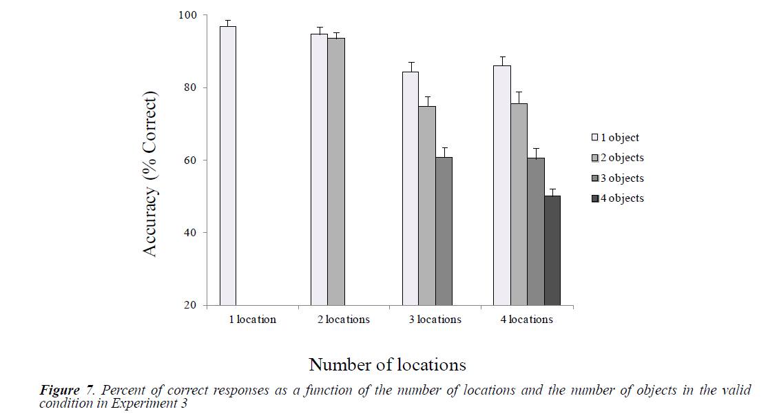
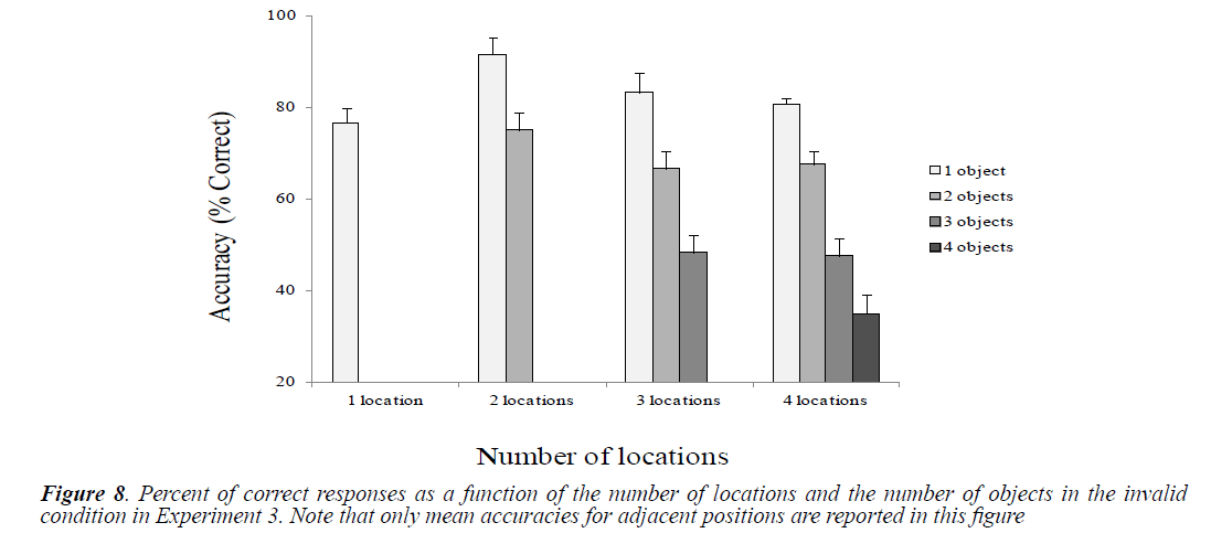
Mean accuracies were calculated as a function of the number of locations and objects in the valid and the invalid conditions (Figures 7 and 8).

The LME analysis was conducted with Number of locations, Number of objects and Validity as a fixed predictors and participants as a random factor. The results showed significant main effects of Number of locations, t (5816)=-5.40, p<0.0001, Number of objects, t (5816)=- 3.93, p<0.0001 and Validity, t (5816)=-3.90, p<0.0001. We found also significant interactions between Number of locations and Number of objects, t (5816)=3.13, p<0.001, between Number of locations and Validity, t (5816)=3.54, p<0.0001, and between Number of objects and Validity, t (5816)=2, p<0.01. The triple interaction between the three factors was also significant, t (5816)=-2.29, p<0.01.

Further analysis regarding the possible presence of mixed effects (i.e., random slopes) did not reveal significant individual differences across participants on the magnitude of the effects of the number of locations, or the number of objects, p_s>0.1. The following analysis focused on the differences between conditions related to the number of locations and objects in the valid and the invalid conditions.

Figure 7.Percent of correct responses as a function of the number of locations and the number of objects in the valid condition in Experiment 3.

Figure 8.Percent of correct responses as a function of the number of locations and the number of objects in the invalid condition in Experiment 3. Note that only mean accuracies for adjacent positions are reported in this figure.

Effects of the Number of Locations and the Number of Objects in the Valid Condition

Paired t-test comparisons were performed to examine differences between conditions related to the number of locations and the number of object (Table 7). Overall, we observed a significant decline in performance in 3 and 4-location conditions compared to 1 and 2-locaion conditions. The pattern of results observed in the 3-location condition is very similar to the one obtained in the 4-location condition. Regarding the effect of the number of objects, we found significant linear performance decay as the number of objects increases in the 3- and the 4-location conditions.

Table 7. Paired t comparisons between experimental conditions in the valid condition in Experiment 3.

Effects of the Number of Locations and the Number of Objects in the Invalid Condition

We performed paired t-test comparisons to analyze differences between conditions related to the number of locations and the number of objects (Table 8). Although not significant, but the higher performance was observed in the 2-location condition. Conversely, the lowest performance level was observed in the 1-location condition compared to 2, 3 and 4-location conditions (in the presence of one object). Furthermore, we observed mostly performance decay as the number of objects increases in the 2, 3 and 4-location conditions. Targets presented at adjacent invalid positions were better identified than those presented at distant invalid positions regardless of the number of locations and objects (adjacent position (1L/1O) vs. distant position (1L/1O), t (9)=3.25, p <0.01; adjacent position (2L/1O) vs. distant position (2L/1O), t (9)=2.8, p<0.05; adjacent position (2L/2O) vs. distant position (2L/2O), t (9)=4.58, p<0.005.

Table 8. Paired t comparisons between experimental conditions in the invalid condition in Experiment 3.

Discussion

Taken as a whole, the pattern of results in Experiment 3 is similar to previous results in Experiments 1 and 2. We observed a significant effect of the number of locations. The performance decayed beyond two locations. Furthermore, we detected a robust effect of the number of objects, especially with three and four locations. However, we didn’t observe any performance drop with two processed objects. Moreover, we systematically obtained a significant effect of validity. Targets presented at valid locations were more accurately detected than targets presented at invalid locations. In the latter, the increase of the number of objects induced decay in performance. The effect of the number of location was less sizable since difference between most conditions wasn’t significant. Nevertheless, we detected performance decay in 1-location condition compared with 2-location condition in which the proportion of targets' identification was clearer.

These findings are in line with those of Experiment 1 where the identification of digits appearing among a set of letters was influenced by a semantic difference between these stimuli. We considered that this semantic contrast allowed an attentional re-allocation over targets when they appeared thereby to facilitate their processing. Similarly, the color contrast in Experiment 3 allowed guiding attentional re-allocation over targets.

The main result is the absence of a difference between 3-location and 4-location conditions which was particularly due to the increase in performance in 3-location condition. Reallocating attention over targets due to the contrast between targets and distracters allowed participants to minimize the attentional allocation difficulty generated by the spatial organization of locations. Therefore, attentional resources spread over 3-location configuration could be concentrated yet again over targets. Furthermore, the introduction of contrast between targets and distractors has resulted in an explicit effect of the increase in objects' number. The latter indicates that the amount of attentional resources allocated over three locations remained lower than the required amount of resources related to the growing perceptual load following the increase in the number of objects.

We also observed a significant improvement in performance in the invalid condition compared to previous experiments. This effect is mainly driven by the colorbased selection process of targets even when attention was previously allocated to valid locations. Nevertheless, even if this color-based selection made such advantage, spatial endogenous attention still able to induce a facilitatory effect since performance was systematically higher in valid relative to invalid conditions.

To sum-up, we found about the same thresholds of attentional allocation and processing observed in the previous experiments. Attentional allocation capacity became less efficient when attention was split into three locations. Objects’ processing became also less efficient when attentional resources were distributed over three locations.

General Discussion

The main question addressed in the present study deals primarily with the dissociation between the costs related to the division of attentional selective allocation in one hand, and that related to multiple objects processing on the other hand. Our results showed a strong effect of the number of locations, which became particularly salient when observers had to split their attention over more than two locations. Moreover, our findings revealed a distinct effect of the number of objects when observers had to process four objects simultaneously after attending to four non-contiguous locations. More importantly, the non-linear decrease in performance showed an interaction between the two factors. Performance did not vary from one to two locations, but showed a reliable decline from two to three or four locations. Similarly, we did not find any effect of the number of objects in the two- and threelocation conditions, but we observed a gradual decline in performance as the number of objects increased with four locations. Furthermore, the results showed a very important decline in performance when the participants had to attend to three locations. This result is very intriguing, especially when we observed an unexpected increase in performance when the participants had to pay attention to four attended locations (for one-object condition).

Number of Locations, Number of Objects and Attentional Capacity

It is well known that the selection of an object is determined by different parameters likely to enhance or not the probability of its processing. An important factor is the separation of the number of locations from the objects present, an idea that was partly addressed by Palmer when he manipulated the set-size effects of stimuli in presence of simple vs. complex visual search tasks [26]. We investigated this factor by manipulating the number of attended locations. Thus, theoretically we can hypothesize that the resources would be more distributed as the number of locations increases. According to the pattern of our results, the probability of processing objects accurately does not vary linearly with the amount of resources distributed over locations. Indeed, we first observed that attending to two locations was accurately performed as the participants had to select a single location, but we found a massive decline in performance when attention had to be allocated to more than two locations. This highlights the existence of a threshold for attentional allocation capacity over space, at which the amount of resources at a specific location becomes insufficient to achieve further processing of the object. We can presume that exceeding the threshold is likely to be accompanied by a loss in spatial resolution at each attended location. Thus, it is conceivable to have as many resources as attentional foci but this division can result in a loss of resolution that can vary depending on the layout of the foci and not just their number. Such lack of resolution would produce a proportional decrease in the amount of visual information that would be extracted from the to-be-processed object [27].

The essential idea to be retained is the presence of a tradeoff between the selection accuracy that is strictly linked to the amount of allocated resources and the number of selected locations. The capacity to process objects is not a monotonic function of such a trade-off. Indeed, the spatial resolution at two attended locations is supposed to be inferior to that at a single location but the processing of objects is achieved with an equivalent accuracy. Such finding is in line with the study of Awh and Pashler, who showed that attention, can be split efficiently over two non-contiguous regions [5].

Although our targets were displayed at 80 ms which make saccades unlikely to be triggered, it is not excluded that participants could make saccades to an attended location during either the 500 ms previewed locations' display or the subsequent 500 ms blank ISI. The latter could bias the distance between attended targets and their cued locations. Therefore, follow-up ERP studies will help address such issue by ruling out trials affected by eye movements.

According to the biased competition framework, we can assume that increasing the number of objects increases the strength of competition between these objects for neuronal representation [28]. The resources required to process a single object are less important than those required to process one object that is within other competing objects, because in the latter case there are less available resources for each object. Thus, one can predict a gradual decline in performance as the number of competing objects increases in the scene. As for the impact of the number of locations, we did not observe any such monotonic decrease in performance. We found only such effect of objects when the participants had to attend to four locations. The data do not reveal this effect even with three attended locations. We will not consider this result because the specific effect of the spatial organization seems to indirectly influence the processing of objects, as we explain in the next section, but we can underline the absence of a manifest cost when two objects have to be processed compared with a single one after attending to two locations. Despite the existence of an additional encoding load imposed by the second competing object, two objects can be processed with the same efficiency as with a single object.

It seems that prior allocated resources towards each location remain sufficient for encoding objects, although firstly, they had been previously divided, and secondly, the processing of objects became more demanding due to their competition. Conversely, when resources were distributed over four locations, the processing of objects became more sensitive to the increasing encoding load of objects. We already supposed an exceeding of the threshold of attentional allocation capacity reflected by insufficient resources at each of the four locations and, therefore, by a marked loss in spatial resolution. This effect is added to the growing required resources to encode competing objects as their number increases. Thus, we can imagine that the least supplementary load is accompanied by a gradual parallel coarseness of corresponding representations. The latter would be extremely coarse when four objects have to be processed. In this case, the resources required to encode each object are largely more important than those required to encode a single object. Then, coarse representations of four objects were transferred into VSTM or as Zhang and Luck pointed out, participants store a high-resolution representation of a subset of objects and retain poorresolution representation or no representation at all about the others [29].

Based on our findings in the present study, attention is likely to be distributed over two locations with an equivalent efficiency as when it was deployed over a single location. Hence, the amount of resources allocated to each of the two locations (suppose 40% of resources to each location) enables the processing of one or two objects with the same efficiency, despite the growing encoding load when two objects have to be processed (suppose that 30% of resources are necessary to encode a single object, and when a second object is added, 40% of resources are required to process each object because of their competition). The division of attention into four locations leads to a large decrease in the resources allocated to each location that exceeds the threshold of capacity (suppose 25% of resources to each one). Thus, even if one object appears at one of these locations, its processing is achieved with a lower efficiency than when it appears after attending to one or two locations (25% of resources are less than the 30% of the required resources).

Increasing the number of to-be-processed objects makes processing more difficult, because the resources required for processing become more important (for example, 40% for each object when processing two objects, 50% when processing three objects, and 60% when processing four objects). In all cases, the processing is less efficient compared with that for one or two attended locations, but this efficiency remains a function of the number of to-beprocessed objects. As the latter increases, the processing efficiency decreases.

Interaction between Attention, Allocation and Processing

Although attentional allocation usually precedes object processing, our results showed that object processing can modulate or narrow initial attentional allocation over objects. In Experiments 1 and 3, the contrast between targets and distractors allowed selective attentional “feedback” over targets’ locations which narrowed attentional allocation. Rauschenberger and Yantis, found, for example, that parts of an occluded object might be initially selected as different objects but after the object identification, they can be reselected as a single integrated object [30]. Consistent with this view, topdown phenomena such as object familiarity or expectation can also modulate the attentional allocation over objects and their subsequent representation [31]. The interaction between these two processes is likely to enable us to perform the most optimal integrated representation of objects.

Spatial Organization Effect

Two unexpected results were found regarding the spatial organization effect. First, we observed a great decline in performance when the participants had to attend to three locations. Second, we did not found any effect of the number of objects in this condition. Intuitively, one may predict a decrease in performance parallel to the increase in the number of locations, regardless of the number of objects. More interestingly, in the presence of one object to-be-processed, accuracy was higher at the 4-location condition than at the 3-location condition.

A possible explanation for this counterintuitive result could be attributed to the nature of spatial organization of objects themselves in our paradigm. Indeed, the spatial configuration involving four locations is characterized by the presence of four symmetrical axes likely to facilitate the attention split over locations, whereas with three locations, only a single axis of symmetry is present in each corresponding spatial configuration (Figure 9).

Several findings suggest that symmetry from multiple axes yields more saliency to the spatial configuration of locations in comparison with symmetry with one axis [23,24,32]. As a result, the saliency of the spatial configuration enables to reduce resource cost and successfully maintain the split of attention over space. In addition, attentional foci can be accurately attended with four locations, which can also limit the selection to these limited spots. On the contrary, spatial configurations with three attended locations do not allow such resources limitations at these locations due to the luck of saliency. Such layout could explain the null effect of the number of objects in this condition. The presence of this unexpected effect of organization that plays different roles in 3-location and 4-location conditions makes the comparison between them uneven. Further investigations would hold constant the number of spatial configuration per condition.

The Gradual Distribution of Attention

The division of attention is characterized by a gradual attentional distribution over space which may have different features given the number of attended locations. According to the attentional gradient model [33], it is well known that attentional distribution can be adjusted from a narrow area of the visual field to a more diffuse deployment across the visual field. When attentional distribution covers a narrow window then the processing of the attended region is detailed and efficient, but the attentional gradient flexibility is reduced. In consequence, the decrease in available resources outside the attended area is significant. Such statement is supported by the low performance observed when participants had to report the object that occupied the adjacent invalid location. In this condition, the gradual attentional falling-off as a function of distance matches the presence of extremely coarse representations of adjacent locations likewise those of distant locations. Conversely, when the attentional distribution is deployed over a large area in the visual field, processing becomes less grained but more extensive, because all attended locations are framed within one wide attentional focus. With this bulky layout, surrounding locations benefit from more resources than in the narrow focus mode. Indeed, we found in the present study a better performance when attention is allocated within a large spatial region containing two, three, or even four potential locations. However, as the number of objects presented at invalid locations increases, the processing becomes shallower. Such effect is likely due to the very low amount of available resources allocated to each invalid location.

The Division of Attention

The present findings could provide also a valuable input to the controversial division of attention debate. Indeed, our data are not in line with the models that restrict attentional distribution to a single spatial region. This conclusion is consistent with some previous investigations [5,7,34-36]. However, at some point, selection and processing of the attended objects showed a gradual loss in efficiency, as we can notice, for example, when attention is split into four locations and when the number of the processed objects increases. Such result merely highlights that the division of attention is not an “all or none” process.

It should be also noted that we have used in our study a more conservative mask than in the original paradigm by Awh and Pashler in order to provide a more stringent test for our hypotheses [5]. Indeed, the consistency of our pattern is obtained with a strong pattern masking reflecting an interruption of the object processing that involves a competition for the higher level mechanisms in object recognition as shown in many studies [37].

Figure 9.Number of symmetry axes within the spatial configuration according to the number of locations.

More importantly, the present study is the first, to our knowledge, to dissociate the effect of the attentional division towards locations and that of the multiple processing of objects. From a methodological perspective, such differentiation has implications for the general debate about the division of attention issue. Indeed, follow-up studies have to carefully specify the nature of the manipulated factors in terms of costs in relation to the number of objects and locations. Furthermore, these two costs could be sensitive to specific parameters. For example, attention allocation over locations could be more efficient when the locations are spatially close [38], whereas multiple processing of objects could be well achieved when the objects are non-contiguous [39]. Similarly, attentional allocation is known to vary as a function of the hemispheric organization [5,10], spatial configuration and the type of the onset of distractors [40]. As for multiple processing, the visual complexity of objects, the requirement of the task, or the required representation resolution can modulate these costs as well [11].

Attentional Allocation, Processing and VSTM

Many studies have shown that the selection and the transfer of information in VSTM are monitored by bottom-up and top-down attentional processes [41-44]. However, even though we know that attending to a particular location or object improves its transfer into VSTM, we do not know exactly how attentional allocation to multiple locations leads to the transfer of multiple corresponding objects in VSTM. Indeed, several distinct mechanisms including detection, identification, and memorization can operate together in the tested task. For instance, to what extent does the memory component contribute to these findings without a VSTM delay? Although, our study did not have as a main goal to assess the capacity of VSTM per se, but it is clear from the data that the implications of dissociating attentional allocation from processing are not restricted to attentional processes. The current results indicate that the VSTM capacity is a consequence of the interaction between these two attentional stages. For example, Jiang et al. showed, VSTM storage could vary as a function of the spatial configuration of locations at the attentional allocation stage [45]. It could also vary according to the complexity of the to-be-retained objects at the processing stage [46] and slow to the temporal characteristic of the display [47].

Limitations

We did not control in the present study for eye movements, since abrupt moves from one target to another can be encouraged by the nature of the used paradigm [48]. Although the issue of eye movements is relevant but many studies in spatial attention suggested that brief durations such as in our paradigm (80 ms) are too short to trigger saccades to multiple locations. However, removing in future follow-up studies all trials contaminated by express saccades may provide a fine-grained level of control [49]. While we opted for an item-based analysis - with sufficient trials per condition - via LME models, increasing the number of participants will further increase the experimental power of the findings. In addition, the presence of many participants will allow further crossexperiment analyses.

Conclusion

Controlling experimentally the effects of the number of locations and the number of objects seems to be a straightforward manipulation to disentangle between the difficulty of distributing our resources over many attended locations and the difficulty of engaging in parallel encoding of many objects. These two factors were not separated, to our knowledge, in previous experiments, which is likely to mask the importance of resources availability over the number of salient objects to pay attention to. Our findings may provide new important theoretical and experimental insights to the controversial attentional division debate.

References

1. Eriksen CW, Yeh Y. Allocation of attention in the visual field. Journal of Experimental Psychology 1985; 11: 583-597.
2. Posner MI. Orienting of attention. Quarterly Journal of Experimental Psychology 1980; 32: 3-25.
3. Heinze H, Luck SJ, Muente TF, Goes A, Mangun GR, et al. Attention to adjacent and separate positions in space: An eletrophysiological analysis. Perception and Psychophysics 1994; 56: 42-52.
4. Pan K, Eriksen C. Attentionaldistribution in the visual field during same-different judgments as assessed by response competition. Perception and Psychophysics 1993; 53: 134-144.
5. Awh E, Pashler H. Evidence for split attentional foci. Journal of Experimental Psychology: Human Perception and Performance 26: 834-846.
6. Bichot NP, Cave KR, Pashler H. Visual selection mediated by location: Feature-based selection of noncontiguous locations. Perception and Psychophysics 1999; 61: 403-423.
7. McMains SA, Somers DC. Multiple spotlights of attentional selection in human visual cortex. Neuron 2004; 42: 834-846.
8. Scharlau I. Evidence for split foci of attention in a priming paradigm. Attention, Perception and Psychophysics 2004; 66: 988-1002.
9. Huang L, Pashler H. A boolean map theory of visual attention. Psychological Review 2007; 114: 599-631.
10. Kraft A, Pape N, Hagendorf H, Schmidt S, Naito A, et al. What determines sustained visual attention? The impact of distracter positions, task difficulty and visual fields compared. Brain Research 2007; 1133: 123-35.
11. Xu Y, Chun MM. Selecting and perceiving multiple visual objects. Trends in Cognitive Sciences, 2009; 13: 167-174.
12. Schneider W, Eschman A, Zuccoloto A. E-Prime reference guide. Psychology Software Tools Inc., Pittsburgh 2002.
13. Baayen HR. Analyzing linguistic data: A practical introduction to statistics. Cambridge University, Press, Cambridge 2008.
14. Baayen HR, Davidson DJ, Bates DM. Mixed-effects modeling with crossed random effects for subjects and items. Journal of Memory and Language 2008; 59: 390-412.
15. Bates DM. Fitting linear mixed models in R. R News 2005; 27-30.
16. Milin P, Filipovic-Durdevic D, Moscoso del Prado, Martin F. The simultaneous effects of inflectional paradigms and classes on lexical recognition: Evidence from Serbian. Journal of Memory and Language 2009; 60: 50-64.
17. Rodríguez-Ferreiro J, Davies R, González-Nosti M, Barbón A, Cuetos F. Name agreement, frequency and age of acquisition, but not grammatical class, affect object and action naming in Spanish speaking participants with Alzheimer's disease. Journal of Neurolinguistics 2009; 22: 37-54.
18. Egeth HE, Santee JL. Conceptual and perceptual components of interletter inhibition. Journal of Experimental Psychology: Human Perception and Performance 1981; 7: 506-517.
19. Estes WK. Similarity-related channel interactions in visual processing. Journal of Experimental Psychology: Human Perception and Performance 1982; 8: 353-382.
20. Massaro DW, Cohen MM. Visual, Orthographic, Phonological, and Lexical influences in reading. Journal of Experimental Psychology 1994; 20: 1107-1128.
21. Miller J. The flanker compatibility effect as a function of visual angle, attentional focus, visual transients, and perceptual load: A search for boundary conditions. Perception and Psychophysics, 1991; 49: 270-288.
22. Paquet L, Lortie C. Evidence for early selection: Precuing target location reduces interference from same-category distractors. Perception and Psychophysics 1990; 48: 382-388.
23. Wagemans J, Van Gool L, d?Ydewalle G. Detection of symmetry in tachistoscopically presented dot patterns: Effects of multiple axes and skewing. Perception & Psychophysics 1991; 50: 413-427
24. Wenderoth P. The effects on bilateral-symmetry detection of multiple symmetry, near symmetry, and axis orientation. Perception 1997; 26: 891-904.
25. Harms L, Bundesen C. Color segregation and selective attention in a nonsearch task. Perception and Psychophysics 1983; 33: 11-19.
26. Palmer J. Set-size effects in visual search: The effect of attention is independent of the stimulus for simple tasks. Vision Research 1994; 34: 1703-1721.
27. Franconeri SL, Alvarez GA, Enns JT. How many locations can you select? Journal of Experimental Psychology 2007; 33: 1003-1012.
28. Desimone R, Duncan J. Neural mechanisms of selective visual attention. Annual Review of Neurosciences 1995; 18: 193-222.
29. Zhang W, Luck SJ. Discrete Fixed-Resolution Representations in Visual Working Memory. Nature 2008; 453 : 233-235.
30. Rauschenberger R, Yantis S. Masking unveils pre-amodal completion representation in visual search. Nature 2001; 410: 369-372.
31. Zemel R, Behrmann M, Mozer MC, Bavelier D. Experience-Dependent Perceptual Grouping and Object-Based Attention. Journal of Experimental Psychology: Human Perception and Performance 2002; 28: 202-217.
32. Palmer SE, Hemenway K. Orientation and symmetry: Effects of multiple, rotational, and near symmetries. Journal of Experimental Psychology: Human Perception & Performance 1978; 4: 691-702.
33. LaBerge D, Brown V. Theory of attentional operations in shape identification. Psychological Review 1989; 96: 101-124.
34. Castiello U, Umiltà C. Splitting focal attention. Journal of Experimental Psychology: Human Perception and Performance 1992; 18: 837-848.
35. Hahn S, Kramer AF 1998. Further evidence of division of attention over noncontiguous visual field. Visual Cognition 5: 217-256.
36. Malinowski P, Fuchs S, Müller MM. Sustained division of spatial attention to multiple locations within one hemifield. Neuroscience Letters 2007; 414: 65-70.
37. Brehaut J, Enns JT, Di Lollo V. Visual masking plays two roles in the attentional blink. Perception & Psychophysics 1999; 61 : 1436-1448
38. Eriksen BA, Eriksen CW. Effects of noise letters upon the identification of a target letter in a nonsearch task. Perception and Psychophysics 1974; 16: 143-149.
39. McCarley JS, Mounts JRW, Kramer AF. Spatially mediated capacity limits in attentive visual perception. Acta Psychologica 2007; 126: 98-119.
40. Kramer AF, Hahn S. Splitting the beam: Distribution of attention over non contiguous regions of the visual field. Psychological Science 1995; 6: 381-386.
41. Cowan N, Morey CC. Visual working memory depends on attentional filtering. Trends in Cognitive Sciences 2006; 10: 139-141.
42. Henderson JM, Hollingworth A. High-level scene perception. Annual Review of Psychology 1999; 50: 243-271.
43. Schmidt BK, Vogel EK, Woodman GF, Luck SJ. Voluntary and automatic attentional control of visual working memory. Perception & Psychophysics 2002; 64: 754-763.
44. Vogel EK, Woodman GF, Luck SJ. Pushing around the locus of selection: Evidence for the flexible selection hypothesis. Journal of Cognitive Neuroscience 2005; 17: 1907-1922.
45. Jiang Y, Olson IR, Chun MM. Organization of visual short-term memory. Journal of Experimental Psychology: Learning, Memory & Cognition 2000; 26: 683-702.
46. Alvarez GA, Cavanagh P. The capacity of visual short-term memory is set both by visual information load and by number of objects. Psychological Science 2004; 15: 106-111.
47. Haladjian HH, Mathy F. A snapshot is all it takes to encode object locations into spatial memory. Vision Research 2015; 107: 133-145.
48. Jans B, Peters JC, De Weerd P. Visual spatial attention to multiple locations at once: The jury is still out. Psychological Review 2010; 117: 637-684.
49. Van der Stigchel S, Nijboer TCW. Spatial Attention and Eye Movements. Neuropsychology of Space, Academic Press, San Diego 2017; 159-196.