Research Article - Journal of Environmental Waste Management and Recycling (2022) Volume 5, Issue 5

Determinants of household solid waste disposal practices in the residential neighborhoods of a rapidly growing urban area in Nigeria

Timothy Ishi^1*, E.M Tyavyar², W.A Nomkpev¹

¹Department of Geography, Benue State School of Health Technology, Agasha, Nigeria

²Federal University of Agriculture Road, Akawe Torkula Polytechnic, Makurdi, Nigeria

*Corresponding Author:

Ishi T
Department of Geography
Benue State School of Health Technology
Agasha, Nigeria
E-mail: timothy.ishi.pg00657@unn.edu.ng

Received: 01-Sep-2022, Manuscript No. AAEWMR-22-73591; Editor assigned: 05-Sep-2022, PreQC No. AAEWMR-22-73591(PQ); Reviewed: 19-Sep-2022, QC No. AAEWMR-22-73591; Revised: 21-Sep-2022, Manuscript No. AAEWMR-22-73591(R); Published: 28-Sep-2022, DOI:10.35841/aaewmr-5.5.121

Citation: Ishi T, Tyavyar E.M, Nomkpev W.A. Determinants of household solid waste disposal practices in the residential neighbourhoods of a rapidly growing urban area in Nigeria. Environ Waste Management Recycling. 2022;5(5):121

Keywords

Determinants, Household, Disposal, Residential, Neighbourhoods.

Introduction

Waste management is one of the most important environmental problems in most countries today including Nigeria. Solid Waste Management (SWM) has been recognized as one of the biggest challenges facing municipal authorities across the world, as a result of population growth, urbanization, and poverty [1-4]. Improving public access to clean and safe solid waste management services is one of the key components of sustainable human development and environmental protection. Yet the amount and quality of solid waste management services in the majority of developing countries are generally insufficient and rudimentary [5]. The waste management sector is crucial to everyone as it protects not only our health, but also the environment. However, rising population, consumerism, economic growth, and urbanization on a global scale has fueled a daunting amount of waste. On average, roughly two billion metric tons of waste is generated globally each year with a per capita generation of 0.74 kg of waste per day. This is expected to increase in the coming decades putting increased pressure on the waste management industry.

Poorly-managed waste can cause flooding, waste landslides, transmits diseases such as cholera and malaria via breeding mosquitos and other respiratory problems through airborne particles due to burning of waste. While East Asia and Pacific region currently produces most of the world’s waste, Sub-Saharan Africa, South Asia, Middle East and North Africa region has the largest growing rate of waste in the next three decades with economic growth and urbanization. Hence, global policy makers have identified proper waste management as an important pre-requisite when achieving sustainable development and included target 5 of SDG Goal12: ‘‘substantially reduce waste generation through prevention, reduction, recycling and reuse (3R)” in the Sustainable Development Goals (SDGs). Since households are responsible for generating wastes, their commitment to proper waste management practices is crucial to achieve the above target.

Accordingly, it is important to understand the drivers behind household waste disposal behaviour in order to introduce effective waste management policies. Many previous studies have explored the household behaviour with regard to waste management in both developed and developing countries. These studies contribute to identify the factors affecting household behaviour with regard to waste disposal and recycling [6-15]. For instance found that education, gender, and age have significant impact on the choice of waste disposal options [6,13]. Moreover, socioeconomic and demographic characteristics such as income, gender and education significantly influence household recycling behavior [15- 17]. Socio-psychological factors such as social and personal norms as well as individual attitudes also affect the recycling behaviour, [7,8,11,14].

An estimated 2 billion people globally do not have access to waste collection services, and 3 billion do not have access to controlled waste disposal [18]. This lack of services and infrastructure has a detrimental impact on public health and the environment with waste being dumped or burnt in communities. In Nigeria, municipalities and other authorities have to deal with increasing volumes of household waste, as of 2018, waste in Nigeria was mainly disposed informally, specifically, around 59 percent of waste was managed informally [19]. Disposal within compound, instead held 29 percent of the total waste management, only about 4 percent of the waste was collected by the Government waste management agencies [19].

There is paucity of research findings on household solid waste disposal status of Makurdi municipality. Although previous studies have noted the imperative of household solid waste management in Makurdi metropolis [20,21] and have argued in favour poor solid waste solid waste management condition of the municipality, the determinants’ of household solid waste disposal in Makurdi metropolis remains unexplored and the quest to develop an empirical evidence of the determinants’ necessitate this study.

Material and Methods

Theoretical model

Based on the concept of [22-25] the logit model for household solid waste disposal status was set up to explain household choice of waste disposal. The model assumes that a household generates utility by consuming environmental goods which depends on a vector of household demographic and socioeconomic characteristics (X). To explain β at household level, households were classified into two categories as the one who dispose solid wastes effectively and ineffectively based on Benue State Environmental law. The logit model for solid waste disposal practice at household level can be specified as:

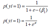
Where:

zi = the function of a vector of explanatory variables

e = the base of natural logarithm

P (yi = 1) = the probability of choosing to dispose solid waste effectively.

Then;

1-P (yi=1) = represents the probability that households’ will not effectively dispose their solid waste and is expressed as:

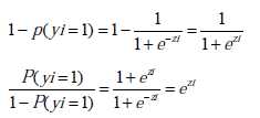
The Above equation simplify us the odds ratio of the probability that a household will be effectively managed to the probability that it will not be effectively managed. Taking the natural log of equation we obtain.

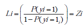
Where:

Li is the log of the odd ratio which is not only linear in the explanatory variables but in the parameters also. Thus introducing the stochastic error term (U_i ) the logit model can be written as

Where = explanatory variables that determines the households’ effective solid waste disposal.

β₀ = constant term

β’_s = coefficients’ to be estimated

Dataset and Sampling Procedure

The households’ data were extrapolated from the projected population census data of 1991, using the national growth rate of 2.9%. The 1991 enumerations areas were carefully superimposed on the residential neighbourhood map with the aid of traditional rulers and relevant stakeholders that were familiar with the communities during the 1991 census. A multistage sampling technique was employed, first, 398 respondents were sampled using Slovins’s formula:

Where:

n = Sample size

N= Total number of households in the study area (89,019)

e= Acceptable error size which is 0.05

1= Constant.

Based on the formula;

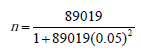
Therefore, the sample size is 398

Bowleys proportional technique was used to determine the number of respondents in each residential neighbourhood, it is given as:

Where;

N= total households population

n= total sample size

h= total household population for each residential neighbourhood

ni= sample size for each residential neighbourhood

Study Area

Makurdi has a total population of 239889 people (NPC, 1991) which was projected to 534,113 in 2019 by the researcher. Makurdi is among the oldest town in North Central Nigeria with a geographic location of 7⁰ 44’ N, 7⁰55 N and 80 20’44’’E and 7⁰40’ 44’’E of the Greenwich meridian as presented in figure 1. It serves as a vital link between the geographic geographical North and South Nigeria to the countries Eastern bloc as such the city is refered to as the microcosm of Nigeria. The town plays a dual role of being the state and local government headquarters. It has a warm and humid climate with a daily average temperature of 37 ⁰ C and mean annual rainfall of 1218 millimeters with a double maxima rainfall regime. During the time of the field survey, the town had 16 residential neighbourhoods (see Figure 1). On the public services front, the supply of housing, water, sanitation and solid waste management falls short of the requirement within the municipality.

Figure 1: Makurdi municipality showing residential neighborhoods.

Results and Discussion

Trends of households’ solid waste disposal practices

As shown in figure 2, Makurdi households predominantly disposed their waste through illegal dumping. Currently, 52.2 percent use this disposal practice while burying and burning of waste accounted for the remaining 48.8 percent waste. This because majority (54.5%) of households in the study area had no formal or even informal system of solid waste collection and as such were compelled to find other ways to get rid of their waste as Benue State Environmental and Sanitation Agency (BENSESA) which is the agency responsible for waste management of the municipality account for only 17.3 percent. The study revealed that even households with waste collection system were compelled to use alternative method of waste disposal in an event where such services were not rendered. This contrary to the waste management law of the State as section 19 (a) states that “no person shall burn or burry refuse on any tenement or open place”. Therefore any method of waste disposal aside what is stipulated in the law is illegal and as such referred here as ‘unapproved methods’ because they are not authorized methods and is considered ineffective disposal.

Figure 2:Waste disposal practices used by households.

It is seemingly clear that householders engage in burning and illegal dumping because these practices are not expensive and easy to operate hence space within the household may be a challenge as well as the stress involved in digging a pit to conceal the waste. Plate 1 shows an example of illegal dump site in Gaadi residential neighbourhood in Makurdi metropolis.

Determinants of household’s solid waste management on effective waste disposal

The logistic regression model specified in the theoretical model was estimated using maximum likelihood estimation technique. The model was estimated to ascertain the effect of household solid waste determinants’ on effective household solid waste disposal status in the study area. The classification table a,b (Block O) output as shown in appendix A includes the intercept (constant). Given the base rates of two options (242/398 = 60.8% that a sampled respondents is ineffective in household solid waste disposal, 156/398 = 39.2% that a sampled respondent is effective in household solid waste disposal) and no other information, the best strategy is to predict for every case (see case processing summary table in appendix C) that a sampled respondent will be ineffective in household solid waste disposal. Using this strategy, the tables shows that such prediction will be correct 60.8% of the time.

About variables in the equation, we observed that the intercept (constant) of the model is log (odds) = -0.439. If we exponentiate the log odds, we find that our predicted odds (Exp (B)) = 0.645. This means that, the predicted odds of the sampled respondents being ineffective in households solid waste disposal is 0.645. Since 156 respondents were observed to be effective in households’ solid waste disposal and 242 ineffective in household solid waste disposal, our observed odds were 156/242. This shows clearly that the model itself have a predictive power to say a respondent selected from a case summary (i.e. 398), has a likelihood of 64.5% to dispose household solid waste ineffectively.

Omnibus Tests of Model Coefficients gives us a chi-square (Likelihood Ratio, LR). The LR statistics is distributed chisquare with i degrees of freedom where i is the number of independent variables. This is used to determine if the model is statistically significant. The chi-square of 116.093 on 10df is significant beyond 0.001. This indicates that the overall model is statistically significant and has performed very well. In other words, the model predicts with high degree of accuracy, the likelihood of a sampled respondents being effective or ineffective in households solid waste disposal in the study area. This explains why chi-square is also known as Likelihood ratio (LR)

Under model summary in appendix A, the -2 log likelihood statistics is 0.001. This statistics measures how poorly or otherwise the model predicts the odds ratio of a sampled respondent disposing household solid waste effectively or ineffectively based on the determinants of household solid waste management in the study area. Theory specifies that the smaller the statistics (-2LL) the better, from the table, the -2LL of 0.001 is extremely small and this shows that the model predicts well the odd ratios of a sampled respondent disposing household solid waste effectively or ineffectively in the study area based on the determinants of household solid waste management. The Nagelkerke R2 of 0.643 implies that 64% variation in the waste disposal status is explained by the determinant of household solid waste management in the study area.

The Hosmer-Lemeshow Test is used extensively to assess the fit of the logistic regression model. The Hosmer-Lemeshow tests the fact that there is a linear relationship between the predictor variables and log odds of the criterion variable. Cases are arranged in order by their predicted probability on the criterion variable. Each of these groups is divided into five groups. Each of these groups is then divided into two groups on the basis of actual score on the criterion variable (see the Contingency Table for Hosmer-Lemeshow Test in appendix A), this result in a 2x5 contingency table. The expected frequency is computed based on the assumptions that there is a linear relationship between the weighted combination of the predictor variables and the log odds of the criterion variable. A chi-square statistic is computed comparing the observed frequencies with those expected under the linear model. A non-significant chi-square (shown in appendix A) indicates that the data fits the model well (Tables 1 and 2).

Table 1.Summary of Explanatory variables and hypotheses.

Table 2. Sample size per residential Neighborhood.

So far, we have been able to show how results from our estimated model that it performs very well, and as such can be used to analyze the relationship between predictor variables and criterion variable (household solid waste disposal status) of the sampled respondents in Makurdi municipality (Figures 3 and 4).

Figure 3:Household waste collection service in makurdi municipality.

Figure 4:Existing illegal dumpsite on a major street of Gaadi residential neighbourhood (photo by the Author, 2020).

It is pertinent to note that, estimated probability for stepwise at last step of the estimation process was put at the classification cut off 0.5 at maximum iteration. The default cut-off probability of 0.5 for this model gives good results. Therefore, P = 0.500 and any predictor variable whose P< 0.500 is significant and its inclusion in the model is not likely to be by chance. Note, again that conventionally, the logistic distribution constrains the estimated probabilities to lie between 0 and 1. The wald chi square statistics test the unique contribution of each predictor in the context of other predictors- that is holding constant other predictors as such eliminating any overlap between predictors. The wald estimates gives the “importance” of the contribution of each variable in the model. The higher the value the more “important” it is. Notice that each predictor meets the conventional 0.05 standard for statistical significance, except SEXHH (X₂), FSIZE (X₅) and HLOCATION (X₇). The study noted that the wald χ² has been criticized for being too conservative, that is, lacking adequate explanatory power. Consequently, no serious emphasis is placed on the use of wald χ² for further analysis of the logistic regression results.

The results from table 3 further indicates that the coefficient on the AGEHH variable (i.e age of household head) is negative (-0.011) correctly signed and statistically significant at 5% level of significance. This implies that the age of household head has influence on the probability of a sampled respondent to dispose household solid waste effectively (note that the objective is to see a respondent household solid waste disposal status change from 1-effective disposal to 0- ineffective disposal as a result of his or her household’ socio-economic and demographic variables otherwise known here as household’ solid waste disposal determinants’.). The P-value of 0.4634 <0.5 indicates the significant nature of this variable in the model. The Exp(B) of 0.611 indicates that a unit change (increase) in the age of a sampled respondent would reduce their likelihood of effective household solid waste disposal by 61.1% the of 1.637 indicates that sampled respondents with age of household head in the studied residential neighbourhoods are 1.637 times more likely to dispose household solid waste effectively.

Findings from table 2 also shows that the coefficient on the SEXHH variable (sex of household head) is positive (0.116) correctly signed and statistically at 10% level of significance. This implies that the sex of household head has influence on the probability of a respondent being effective in household solid waste disposal. The P-value of 0.653> 0.5 shows that the inclusion of the variable (SEXHH) was by chance but should not be removed. The Exp(B) of 0.123 indicates that the odds of a sampled respondents disposing household solid waste effectively is 12.3% dependent on the sex of household head. Again, the of 8.130 shows that the sampled respondents are 8.130 times more likely to dispose household solid waste effectively depending on the sex of household head.

The parameter estimates for the household income (HINCOME) on household solid waste disposal is correctly –positively signed (0.138) and statistically significant at 5% level of significance. This implies that household income has influence on the odds or probability of a sampled respondents being effective in household solid waste disposal. The P- value of 0.1378 <0.5 further strengthen the significant nature of HINCOME in explaining the household solid waste disposal status of sampled respondents as purchasing power plays a major role in paying for any environmental goods. The Exp (B) ratio of 0.614 indicates that the probability of a sampled respondents disposing household solid waste effectively can be explained by 61.4% by a unit increase in the household income. The statistics of 1.629 showed that a sampled respondent is 1.629 times likely to dispose household solid waste effectively.

The parameter estimates of YSTAY (i.e years of stay) of the respondent is negatively incorrectly signed (-0.047), but statistically significant at 5% level of significance. This means that years of a sampled respondent in the residential neighbourhood would tend to increase his or her ineffective waste disposal status. This may be due to the fact that the more a sampled respondent stays in an area the more the affinity to dispose household solid waste indiscriminately as field observations reveals that there is almost near absence of community skips (transfer stations) to enable residents effectively dispose their household solid waste hence they result to self-help by using alternative means of waste disposal. The P- value of 0.009<0.5 indicates that the parameter estimates of YSTAY is significant and its inclusion in the model is not by chance. The Exp (B) value of 0.954 showed that the odds of sampled respondents disposing household solid waste effectively will be explained by 95.4% by their years of stay. The of 1.048 statistic indicates that the sampled respondents are 1.048 times more likely to dispose household solid waste effectively by their YSTAY.

The family size (FSIZE) of sampled respondents has a positiveincorrectly signed (0.010) relationship with household solid waste disposal status in the study area, and is not statistically significant. This is because the amount of waste generated per person in a household and subsequent disposal may not necessarily dependent on the number of persons living in the household. The obvious reason is that household solid waste disposal may be independent to family size. Therefore, there is a need to move beyond family size as a quick indicator for effective household solid waste disposal. This means that family size of sampled respondents does not have influence on the waste disposal status of the household. The P-value of 0.9017>0.5 showed that the inclusion of the variable FSIZE in the model is by chance but should not be removed.

The coefficient of level education of household head (EDUHH) of a sampled respondent has positive-correctly signed (0.134) and statistically significant at 5% level of significance. This implies that the EDUHH has influence on the probability of sampled respondent to dispose household solid waste effectively. The Exp(B) statistic of 0.874 affirms that the odds of sampled respondent disposing household solid waste effectively could be explained 87.4% by the level of education attained by the household head. The value of 1.144 also shows that sampled respondents are more likely to dispose household solid waste effectively by 1.144 times. The P-value of 0.314<0.5 shows that the presence of the variable EDUHH into the model is significant and not by chance.

The parameter estimates of household location distance from main road (HLOCATION) of sampled respondent for household solid waste disposal is correctly- negatively signed (-0.40) but not statistically significant. This implies that even though the parameter (HLOCATION) agrees with solid waste management theory, the variable is not significant in explaining the solid waste disposal status of sampled respondents in the study area. Again, the ExP(B) value of 0.001 further indicates that the odds of a sampled respondents disposing household solid waste effectively is 0.001 to household location distance from main road. This explains why we have a larger number of times (1000) a sampled respondent disposing household solid waste effectively by its location distance from main road (HLOCATION).

The coefficient for household willingness to pay for solid waste management service (HWTP) of a sampled respondent is correctly-positively signed (1.692) and statistically significant at 1% level of significance, which implies that, HWTP has influence on the probability of a sampled respondent disposing household solid waste effectively. The Exp (B) statistic of 0.814 again showed that the odds of a sampled respondents disposing household solid waste effectively could be explained 81.4% by ability of respondents to pay for household solid waste management service. The P-value of 0.0001<0.5 also indicates that the estimates is significant in explaining the respondents household solid waste disposal status from effective to ineffective. The value of 1.229 indicates that the sampled respondents’ are 1.229 times more likely to dispose household solid waste effectively by HWTP for solid waste management service in the study area.

The coefficient of awareness to solid waste management (AWARENESS) is positively-correctly signed (1.560) and statistically significant at 5% level of significance. This shows that the awareness to solid waste management has effect on the likelihood of a sampled respondent disposal status. The P-value of 0.0001<0.5 further strengthen the fact that the parameter estimate is significant and its inclusion in the model is not by chance. The Exp (B) value of 0.210 indicates that the odds of a sampled respondents disposing household solid waste effectively can be 21% explained by its awareness to solid waste management in the study area. Again, the value of 4.761 shows that the sampled respondent is 4.761 times more likely to dispose household solid waste effectively if there is an increase in the respondent level of awareness to solid waste management.

Lastly, the parameter estimate of means of transportation of household solid waste to disposal point (MHTRAN) is correctly-positively signed and statistically significant at 5% level of significance. This implies that MHTRAN exert an influence on the probability of a sampled respondent disposing household solid waste effectively. The p-value of 0.0016<0.5 also shows that the estimate is significant and the variable’s inclusion in the model is not by chance. The Exp (B) value of 0.688 revealed that the odds of a sampled respondents disposing household solid waste effectively could be 68.8% explained by his or her means of transporting household solid waste, again, the statistic of 1.454 indicates that a sampled respondent 1.454 times more likely to dispose household solid waste effectively by an increase in the respondents ability to own a means of transporting household solid waste in the study area.

Thus, given that the likelihood ratio (LR) is 116.093 and its P-value at classification cut-off of 0.5, we observe very clearly that LR (116.093) is greater than P (0.5). Therefore, we conclude that household solid waste determinants’ have significant relationship with effective household solid waste disposal of sampled respondents’ in Makurdi Muncipal area of Benue State, Nigeria. The Nagelkerke R2 value of 0.643 (64.3%) shows that households’ solids waste determinants has influence on the household solid waste disposal status in the study area.

Checking multicollinearity and correlation between pairs of variables

Table 3 is known as correlation matrix. It lists the variables names (X1-X10) down the first column and across the first row. The diagonal of the correlation matrix (i.e. the numbers that go from the upper left corner to the lower right) always consists of ones, which shows that they are the correlation between each variable and it self (i.e. a variable is perfectly correlated to itself). In the correlation matrix above (like in every other correlation matrix), there are two triangles that have the values below and to the left of the diagonal (lower triangle) and above to the right of the diagonal (upper triangle). When a matrix such as the one in table 3 has this mirror- image above and below the diagonal it is referred to as a symmetric matrix.

Variables	Coefficients	S.E.	Wald	Df	Sig.	Exp(B)		P-Value
AGEHH (X1) SEXHH (X2) HINCOME (X3) YSTAY (X4) FSIZE (X5) EDUHH (X6) HLOCATION(X7) HWTP (X8) AWARENES (X9) HMTRAN (X10) Constant	-.011	.015	.503	1	.047**	.611	1.637	0.4634
	.116	.258	.203	1	.065*	.123	8.130	0.6530
	.138	.093	2.181	1	.014**	.614	1.629	0.1378
	-.047	.018	6.920	1	.009**	.954	1.048	0.0090
	.010	.081	.014	1	.904	.990	1.010	0.9017
	.134	.133	1.023	1	.031**	.874	1.144	0.3137
	-.040	.122	.109	1	.741	.001	1000	0.7430
	1.692	.346	23.880	1	.000***	.814	1.229	0.0001
	1.560	.323	23.300	1	.000***	.210	4.761	0.0001
	.373	.118	9.942	1	.002**	.688	1.454	0.0016
	4.656	1.032	20.357	1	.000	105.223

Table 3.Resultsonvariables’Coefficients,S.E.,WaldTest,Sig,Exp(B), and P-Value.

Table 4 is used to test multicollinearity indicated by correlation between variables of 0.6, 0.7 and above; and the correlation between pairs of variables. At a glance there is absence of multicollinearity in the model results. The coefficients of correlation express the degree of linear relationship between the row and column variables of the matrix. The closer the coefficient is to zero, the less the relationship; the closer to one, the greater the relationship. A negative sign indicates that variables are inversely related. To interpret a coefficient, square it and multiply by 100. This will give the percent variation in common for the data on the two variables.

Table 4.A 10 Variable Correlation Matrix

The coefficient of correlation between age of household head (AGEHH=X1) and sex of household head (SEXHH=X²) is 0.182 which indicates a low but positive relationship between AGEHH (X1) and SEXHH (X2). Again, the correlation of 0.182 between AGEHH(X1) and SEXHH(X2) means that 0.182² X 100 = 3.3124 percent of the variation of the 398 sampled on these two characteristics (variables) is common. This implies that 3.3124% of AGEHH of the sampled respondents can be predicted from their SEXHH. Furthermore, the synergy between X1 and X2 is likely to make a sampled respondent dispose household solid waste effectively by 3.3124 times.

Table 4 further shows a low but positive relationship between SEXHH (X2) and HINCOME (X3) of 0.058. This implies that the correlation of 0.058 between X2 and X3 means that 0.0582 × 100 = 0.3364 percent of the variation of the 398 sampled respondents on these two characteristics is common. This also implies that 0.3364% of SEXHH (X2) of the sampled respondents can be predicted from their HINCOME (X3). This synergy between X2 and X3 shows that a sampled respondent is 0.3364 more likely to dispose household solid waste effectively by his or her SEXHH and HINCOME.

Table 4 also indicates that there is high positive correlation between HWTP(X8) (i.e household willingness to pay) and EDUHH(X6) (i.e education of household head) of the sampled respondents indicated by 0.840. The correlation between of 0.840 between X8 and X6 means that 0.840² × 100 = 70.56 percent of variation of the 398 sampled respondents on these two variables is in common. This shows that 70.56 percent of HWTP (X8) of the respondents can be predicted from their EDUHH (X6) and vice versa. This synergy between X8 and X6 shows that a sampled respondent is 70.56 times more likely to dispose household solid waste effectively by his or her HWTP(X8) and EDUHH(X6).

If we assume that the sample of determinants’ for households’ solid waste management is random, and the 399th were randomly added to the sample and only his or her SEXHH (X2) were known, then his or her AGEHH (X1) could be predicted by 3.312 percent and HINCOME(X3) within 0.3364 percent of the true value. The reader can peruse table 3 and the relationship between other pairs and the interpretation is the same.

Conclusion

The study has demonstrated that households’ socio-economic variables plays a vital role in sustainable solid waste disposal across the residential neighbourhoods of Makurdi metropolis, north central Nigeria. Evidence from the sixteen residential neighbourhoods shows that there is high level of ineffective and unsustainable household solid waste disposal practices as a result of inadequate solid waste management practices in the study area. The study further shows that the solid waste management authority of the municipality (BENSESA) is overwhelmed with the situation as only a small fraction of household solid waste generated in the municipality were collected by the authority while majority of the waste remains uncollected causing residents to resort to self-help. The absence of government designated solid waste collection points worsen the situation resulting to the proliferations of unapproved disposal sites scattered all over the municipality. To tame this ugly trend, government should create household solid waste collection points in all the sixteen residential neighbourhoods for a more effective robust solid waste collection in the municipality. This can be achieved through the provision of community/street collection containers at the collection points at strategic locations closer to the households they intended to serve as well as partnering with other relevant waste management stakeholders for effective and sustainable service delivery.

Appendix A

Logistic Regression for determinants’ of household solid waste Disposal.

(DataSet1) C:\Users\Timothy Ishi\Desktop\Timothy Terver Data.sav

Block 0: Beginning Block

References

1. Hoornweg D, Bhada-Tata P. What a waste: a global review of solid waste management.

Indexed at, Google Scholar

2. Tacoli C. Urbanization, gender and urban poverty: paid work and unpaid carework in the city. Human Settlements Group, International Institute for Environment and Development; 2012.

Google Scholar

3. UN (2016): The millennium Development Goals report of 2015 on SSA.
4. Desa UN. World urbanization prospects, the 2011 revision. Population Division, department of economic and social affairs, United Nations Secretariat. 2014.

Google Scholar

5. Egbu A, Okoroigwe D. Informal collection of household solid waste in three towns of Anambra State, Nigeria. Present Environment and Sustainable Development. 2014;27(2):101-16.

Indexed at, Google Scholar, Cross Ref

6. Abebaw D. Determinants of solid waste disposal practices in urban areas of Ethiopia: a household-level analysis. Eastern Africa Social Science Research Review. 2008;24(1):1-4.

Indexed at, Google Scholar, Cross Ref

7. Meneses GD, Palacio AB. Recycling behavior: A multidimensional approach. Environ Behav. 2005;37(6):837-60.

Indexed at, Google Scholar, Cross Ref

8. Barr S. Factors influencing environmental attitudes and behaviors: A UK case study of household waste management. Environ Behav. 2007;39(4):435-73.

Indexed at, Google Scholar, Cross Ref

9. Bezzina FH, Dimech S. Investigating the determinants of recycling behaviour in Malta. Manage Environ Qual : Int J. 2011;22 (4), 463–485.

Indexed at, Google Scholar, Cross Ref

10. Sorkun MF. How do social norms influence recycling behavior in a collectivistic society? A case study from Turkey. Waste Manage. 2018;80:359-70.

Indexed at, Google Scholar, Cross Ref

11. Srun P, Kurisu K. Internal and external influential factors on waste disposal behavior in public open spaces in Phnom Penh, Cambodia. Sustainability. 2019;11(6):1518.

Indexed at, Google Scholar, Cross Ref

12. Yokoo HF, Kawai K, Higuchi Y. Informal recycling and social preferences: Evidence from household survey data in Vietnam. Resour Energy Econom. 2018;54:109-24.

Indexed at, Google Scholar, Cross Ref

13. Adzawla W, Tahidu A, Mustapha S, et al. Do socioeconomic factors influence households’ solid waste disposal systems? Evidence from Ghana. Waste Manage Res. 2019;37(1):51-7.
14. Khan F, Ahmed W, Najmi A. Understanding consumers’ behavior intentions towards dealing with the plastic waste: Perspective of a developing country. Resour Conserv Recycl. 2019;142:49-58.

Indexed at, Google Scholar, Cross Ref

15. Alhassan H, Kwakwa PA, Owusu-Sekyere E. Households' source separation behaviour and solid waste disposal options in Ghana's Millennium City. J Environ Manage. 2020;259:110055.

Indexed at, Google Scholar, Cross Ref

16. Ekere W, Mugisha J, Drake L. Factors influencing waste separation and utilization among households in the Lake Victoria crescent, Uganda. Waste Manage. 2009;29(12):3047-51.

Indexed at, Google Scholar, Cross Ref

17. Dwivedy M, Mittal RK. Willingness of residents to participate in e-waste recycling in India. Environ Dev. 2013;6:48-68.

Indexed at, Google Scholar, Cross Ref

18. Yakubu ja. The waste management system in low income areas of jos, nigeria: the challenges and waste reduction opportunities: appendices (doctoral dissertation, university of brighton).

Indexed at, Google Scholar

19. Statistica Research Department (www.statistica.com) (2022).
20. Sha’Ato R, Aboho SY, Oketunde FO, et al. Survey of solid waste generation and composition in a rapidly growing urban area in Central Nigeria. Waste Manage. 2007;27(3):352-8.

Indexed at, Google Scholar, Cross Ref

21. Ishi, T.T (2021). Patterns and determinants of household solid waste management in Makurdi Municipal area of Benue State, Nigeria. Unpublished Ph.D. thesis, University of Nigeria Nsukka.
22. Fefa J. Cassava processing and marketing as poverty fighter in Benue State. Saarbricken, Germany: Lambart Academic Publishing. 2014.

Indexed at

23. Greene WH, Hensher DA. A latent class model for discrete choice analysis: contrasts with mixed logit. Transportation Research Part B: Methodological. 2003;37(8):681-98.

Indexed at, Google Scholar, Cross Ref

24. Gujarati DN. Basic Econometrics. 3-rd ed.

Indexed at, Google Scholar

25. UN-HABITAT. The State of the World's Cities Report 2012/13.