- Biomedical Research (2013) Volume 24, Issue 1
Analytical and Numerical Evaluation of Steady Flow of Blood Through Artery.
N. Sedaghatizadeh1*, A. Barari2, Soheil Soleimani3, M. Mofidi41Department of Mechanical Engineering, Iran University of Science and Technology, Narmak, Tehran, Iran
2Department of Civil Engineering, Aalborg University, Sohngårdsholmsvej 57, 9000 Aalborg, Aalborg, Denmark
3Department of Mechanical engineering, Babol University of Technology, Babol, Iran
4Department of Civil Engineering, Sharif University of Technology, Tehran, Iran
- *Corresponding Author:
- N. Sedaghatizadeh
Department of Mechanical Engineering
Iran University of Science and Technology
Narmak, Tehran
Iran
Abstract
Steady blood flow through a circular artery with rigid walls is studied by COSSERAT Continuum Mechanical Approach. To obtain the additional viscosities coefficients, feed forward multi-layer perceptron (MLP) type of artificial neural networks (ANN) and the results obtained in previous empirical works is used. The governing filed equations are derived and solution to the Hagen-Poiseuilli flow of a COSSERAT fluid in the artery is obtained analytically by Homotopy Perturbation Method (HPM) and numerically using finite difference method. Comparison of analytical results with numerical ones showed excellent agreement. . In addition microrotation and the velocity profile along the radius are obtained by using both numerical and analytical approaches.
Keywords
Blood flow; artery; Cosserat continuum; viscoelastic response; non-Newtonian
Introduction
Over 20 million people die every year due to blood related diseases [1]. Since the blood flow is an important subject in biomedical and medicine sciences, the behavior of blood in the artery is one of the most important problems in biomechanical engineering. Thus many studies have been performed analytically, numerically and experimentally to determine the blood behavior and its different properties [1-5]. The phenomena which are associated with flow of blood through arteries such as pulsatility of flow, non-Newtonian behaviour of blood as a fluid and flexibility of the arteries wall are very complicated; therefore, theoretical study of blood flow is a very difficult problem to attack. The nonlinear behavior of blood was unknown until the second half of the last century [6]. From the rheological point of view, blood is a water based solution which is the combination of organic and inorganic substances and a variety of suspended cells mainly red cells which strongly affects the dynamic of blood as flood so that blood can be characterized as a non- Newtonian fluid [7, 8].Fig. 1 shows the component of a blood sample [7]. Detailed information can be found in previous literatures [6-8].

Figure 1: Components of a blood sample
Experimental studies revealed that the blood viscosity decreased with an increase in shear rate and that blood has a small yield stress. Some constitutive models have been proposed for blood as a non-Newtonian fluid by several researchers. Casson proposed a model which is applied successfully for analysis of blood flow by Merrill and others later [8]. Biviscosity model is another model, which express that blood behaves as non-Newtonian fluid in small shear rates and Newtonian fluid in large shear rates. Nakamura and Sawada used this model successfully [9,10]. In the case of blood flow because of considerable mechanical properties which is emanate from its microstructure, the theory of simple materials cannot solve the problem, so a more sensitive continuum theory such as nonlocal, micropolar, multipolar, and gradient theories [5,11,12] with higher kinematic status will be applied more successfully. The idea of a material body endowed with both translational and rotational degrees of freedom stems from the seminal work of the Cosserat brothers (Cosserat and Cosserat) [13, 14]. In this continuum, the effect of couples and forces are considered independently from each other which later named micropolar continuum by Eringen [11]. Fluids of this continuum medium can support the couple stress, the body couple and nonsymmetric stress tensor and possess a rotation field, which is independent of the velocity field. The rotation field is no longer equal to the half of the curl of the velocity vector field. Because of the assumption of infinitesimal rotations, we can treat the rotation field as a vector field. The theory, thus, has two independent kinematic variables; the velocity vector V and the spin or microrotation vector ω .
Because of complex rheological behavior of blood flow and the fact that blood contains a variety of cells with a spinning movement that affects the blood flow velocity, we should applied Cosserat continuum model. This model can consider the effects of rotational movement and has the ability to describe the complex fluid flows such as non-Newtonian and turbulent fluid flow [11, 12, 15, and 16]. Recently
Sedaghatizadeh et. al [17] conducted a semi empirical semi numerical study on blood flow through an artery in Cosserat continuum, and revealed that the blood flow exhibits a parabolic trend. They also calculated the non- Newtonian factors exist in governing equations using PSO algorithm and find out that these factors are not constant during a cycle of a heart [17].
Equation of motion in Cosserat continuum
In Cosserat continuum both velocity and rotation vector field are considered at any material point. In order to develop the relation between current state of orthonormal directions attached to each material point and its initial state we have the following.
 (1)
(1)
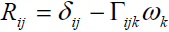
Where  and
and  are the Kronecker delta and permutation
tensor, respectively. The associated Cosserat deformation
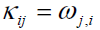
tensor εij and torsion-curvature tensor kij are
written as
are the Kronecker delta and permutation
tensor, respectively. The associated Cosserat deformation
tensor εij and torsion-curvature tensor kij are
written as
 (2)
(2)
 (3)
(3)
where the comma denotes partial differentiation. It is obvious that in the absence of the rotation vector ω , the classical continuum mechanics is recovered
It is assumed that the transfer of interaction between two particles of the continuum through a surface element ni ds occurs by means of both a traction vector ti ds and a moment vector mi ds . Surface forces and couples are represented by the generally nonsymmetric force-stress and couple stress tensor tij and mij , respectively. The balance of linear momentum and angular momentum require that the following equations must be satisfied
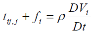 (4)
(4)
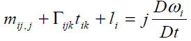 (5)
(5)
Where ρ j,fi and li are the mass density, microinertia, body force per unit mass and body couple per unit mass, respectively, and D Dt denotes the material time derivative. Here we choose linear constitutive equations which describe our material behavior. It can be considered as generalization of Newtonian fluids in the classical Navier-Stockes theory, which are
 (6)
(6)
 (7)
(7)
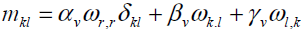
Where π is the thermodynamic pressure. The linear constitutive equation for nonsymmetric stress tensor (i.e. Cauchy's stress tensor), contains an additional viscosity coefficient kv. The value of kv shows the influence of the microrotation field on the stress tensor. The linear constitutive equation for couple stress also contains three additional viscosity coefficients αv , βv and γv.
At this stage the above equations should be combined to obtain the governing field equations. The field equations for micropolar fluids in the vectorial form are given by conservation of mass (i.e. continuity equation)
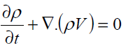 (8)
(8)
Balance of liner momentum
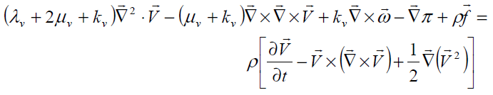 (9)
(9)
And balance of angular momentum
 (10)
(10)
Problem Definition
Fig. 2 shows a part of the femoral artery of a dog where the measurements were made previously at USC School of Medicine. The pressure drop through the artery is measured using two small branch arteries. To simplify the geometry the vessel (Fig. 2.a) assumed and kept to be relatively straight with mild taper (Fig. 2. b). The flow through a vessel is determined by pressure gradient, which is assumed to be constant in most of the problems with practical importance and the vessel is considered as a pipe with radius of R . The Oz axis overlaps the centerline of pipe. In this case the velocity components and the microrotation velocities become
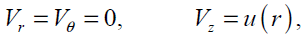 (11)
(11)
 (12)
(12)

Figure 2: a) X-ray tracing of portion of the femoral artery of a living dog. Ligated small branch arteries are marked port No. 1 and 2 [8], b) simplified model of artery.
From continuity when ρ = const [6], we have  By neglecting the body forces and body
couples, the equations of motion (i.e., Eqs. (9) and (10))
are reduced to the following form in cylindrical coordinate
system.
By neglecting the body forces and body
couples, the equations of motion (i.e., Eqs. (9) and (10))
are reduced to the following form in cylindrical coordinate
system.
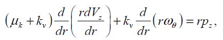 (13)
(13)
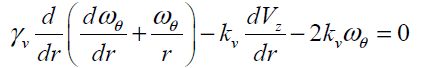 (14)
(14)
The above two coupled partial differential equations should satisfy the following boundary and initial conditions
At 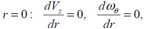 (15)
(15)
At 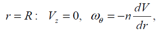 (16)
(16)
where  is a dissipative boundary condition
[11, 18] and 0 ≤n ≤1. This factor is small for a laminar
flow and is increases as flow become turbulent.
is a dissipative boundary condition
[11, 18] and 0 ≤n ≤1. This factor is small for a laminar
flow and is increases as flow become turbulent.
Analysis of the Homotopy Perturbation Method
Homotopy Perturbation Method (HPM) [19-29] is based on the Homotopy which is an important part of the topology [30-31].
 (17)
(17)
with the following boundary condition:
 (18)
(18)
where A is a general differential operator, B a boundary operator, f (r) a known analytical function and Γ is the boundary of the domain Ω. A can be divided into two parts which are L and N, where L is linear and N is nonlinear. Eq. (17) can therefore be rewritten as follows:
 (19)
(19)
Homotopy perturbation structure is shown as follows:
 (20)
(20)
where,
 (21)
(21)
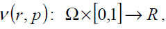
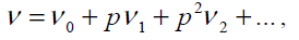
In Eq. (21),p∈[0,1]is an embedding parameter and μ0 is the first approximation that satisfies the boundary condition. We can assume that the solution of Eq. (21) can be written as a power series in p, as following:
 (22)
(22)
and the best approximation for solution is:
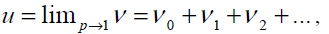 (23)
(23)
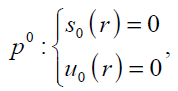
In order to solve Eq. (17) using HPM, we construct the following homotopy; we need an initially condition which is Eq. (18). After constructing the Homotopy Perturbation of Eqs. (13) and (14) and rearranging based on powers of p-terms, we can obtain:
 (24)
(24)
 (25)
(25)
 (26)
(26)
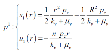
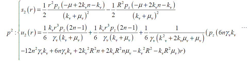
So Vz and wq can be obtained as follows with four terms of approximation as
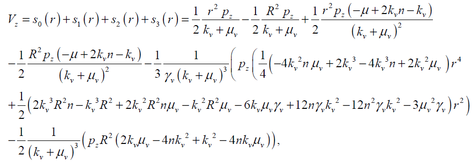 (27)
(27)
and
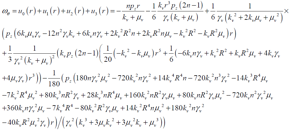 (28)
(28)
In the above solution, the viscosity coefficients of COSSERAT medium ( kv , αv , βv,γv) are unknown. Thus the feed forward multi-layer perceptron (MLP) type of artificial neural networks (ANN) can be employed to calculate these coefficients on the basis of experimental data. In this study, the flow field and the results of experiments done in Fachhochschule Frankfurt by Silber [30] on steady blood flow through a dog artery with the diameter of 12 mm, is considered to determine the viscosity coefficients.
Results and Discussion
In this study Homotopy Perturbation and Finite Difference Methods are implemented to study the steady blood flow through a circular artery. Results are compared in Figs. 6 and 7 for both normalized microrotation and velocity, respectively. As it is obvious analytic outcomes are in good agreement with numerical ones.
Numerical solutions of governing coupled Eqs. (13) and (14) with boundary conditions (15) and (16) are obtained by finite difference FORTRAN code. Successive under relaxation (SUR) method is implemented to solve linear algebraic equations and the value of 0.1 is taken for under-relaxation parameter. The governing equations are discretized by applying second-order accurate central difference schemes. Grid independency was verified on different node numbers from 51 to 201 and finally the number of grid points is taken as 101 along the radius of artery. The convergence criterion (maximum relative error in the values of the dependent variables between two successive iterations) was set at10-10.
To obtain the additional viscosities coefficients, feed forward multi-layer perceptron (MLP) type of artificial neural networks (ANN) and the result obtained in [30] is used in this work.
5.1. Modeling using MLP-type neural networks
An example of a MLP type of neural network with one input node, a single hidden layer with two neuron and one output neuron is shown in Fig.3. An additional input called bias with constant value of 1 is added to the previous input node which works as a shift operator. Each input node is related to each neuron in hidden layer by a connecting weight. The sum of the products of the weights and the inputs is calculated by each neuron in hidden layer and then treated by an activation function. The obtained result is then multiplied by the associated weight C3 and again the previous procedure will be repeated in the output neuron. In the present study hyperbolic tangent and linear functions are used as the activation functions in the hidden and output layers respectively.

Figure 3: Architecture of a network with one hidden layer containing two neurons and one neuron in the output layer
The final output of the current network is calculated as
 (29)
(29)
where,
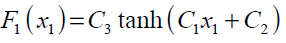 (30)
(30)
Once the number of layers and the number of neurons in each layer, have been selected, the network's weights must be adjusted to minimize the prediction error made by the network. This is the general role of the training algorithms. In this investigation Back-propagation (BP) method is applied to train the ANN which is the most widely used learning process in neural networks today.
Back-Propagation algorithm
Back-propagation was firstly proposed by Werbos [33] which is based on searching an error surface (error as a function of ANN weights) using the gradient descent algorithm for points with minimum error. Consider a network with one hidden layer and one output neuron as shown in Fig 4. When a set of input data (input vector) are propagated through the network, for the current set of weights there is an output Est . The training of perceptron is a supervised learning algorithm where weights are adjusted to minimize the absolute error between the estimated output Est of network and the desired output Des whenever the estimated output does not match the desired output. If the network error ( NE ) is defined as

Figure 4: A feed forward multi-layer perceptron type of neural network with one hidden layer.
Network Error = Est - Des = NE (31)
The training algorithm should adjust the weights to minimize NE2 . For this purpose an artificial neuron with its basic elements is considered as shown in Fig .5.

Figure 5: Basic elements of an artificial neuron
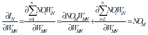
The neuron consists of three basic components; weights, a summing junction and an activation function. The outputs of n neurons NO1,..., NOn lead in neuron N as the inputs. If neuron N is in the hidden layer then this is the input vector of the network. These outputs are multiplied by the associated weights W1N ,..., WnN.The summing junction adds together all these products to provide the input IN for activation function of neuron N . Then IN passes through the activation function AF ( ) and gives the final output of neuron N , which is NON . To commence the calculations, consider neuron M and weight WMN which connects the two neurons. The equation for weight update is as follows:
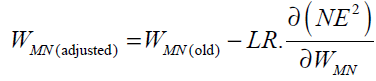 (32)
(32)
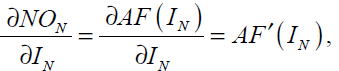
where LR is the learning rate parameter and  is error gradient with reference to the
weight WMN. The chain rule gives
is error gradient with reference to the
weight WMN. The chain rule gives
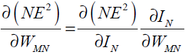 (33)
(33)
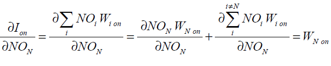
since the rest of the inputs to neuron N are independent of the weight WMN we have
 (34)
(34)
Eqs. (32), (33) and (34) give
 (35)
(35)
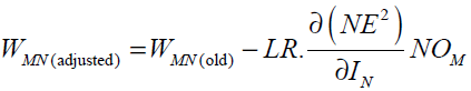
For the case N is an output neuron we have:
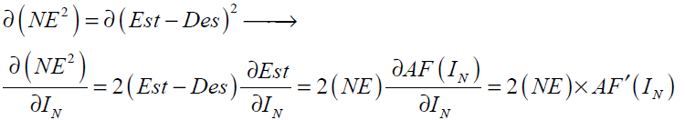 (36)
(36)
Substituting Eq. (36) into Eq. (35) gives
 (37)
(37)
For hyperbolic tangent and linear activation functions AF'(IN ) and the final form of weight update rule can be written as follows:
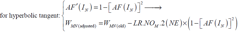 (38)
(38)
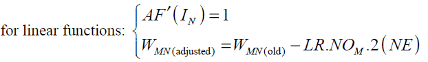 (39)
(39)
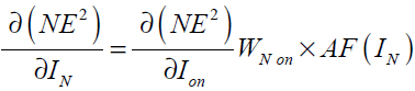
When N is a hidden layer neuron
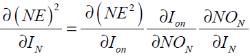 (40)
(40)
where the subscript on represents the output neuron. In Eq. (40) we have
 (41)
(41)
substituting Eq. (41) into Eq. (40) gives
 (42)
(42)
In Eq. (42), is now written as a function of
 which was calculated in Eq. (36).
Hence the weight update rule for a hidden layer neuron takes the following form
which was calculated in Eq. (36).
Hence the weight update rule for a hidden layer neuron takes the following form
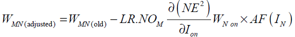 (43)
(43)
The most common parameters for evaluation of a neural network’s performance are minimum total squared errors (or RMS error) and minimum total absolute error (or MAE error). MAE and RMS errors are defined as
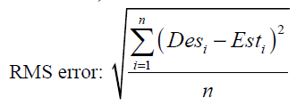 (44)
(44)
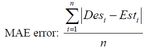 (45)
(45)
where n is the number of training data. The number of hidden layers and the neurons in each of them should be determined in a way to minimum the above errors.
The velocity profile along the radius is shown in Fig. 6. The diagram shows that the velocity has a parabolic trend and change from maximum value at center to zero at the wall. Microrotation is illustrated in Fig. 7 and it shows that, it varies linearly along the radius.

Figure 6: Microrotation profile along the radius

Figure 7: Velocity profile along the radius
The maximum values of V and ω (Vmax, ωmax) can be obtained analytically by substituting r = 0 and r = R in Eqs.(27, 28) respectively as follows:
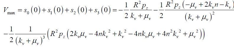 (29)
(29)
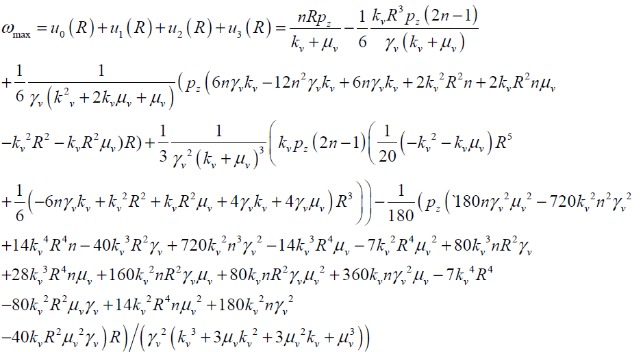 (30)
(30)
Conclusions
In this study a flow simulation respect to time and dimensionless radius based on Cosserat model for a complex fluid like blood has been performed. ANN is applied to obtain the non-Newtonian coefficients. Using these values, the velocity and rotation profiles are calculated over radius of the artery are obtained. The obtained results show that, the maximum values of velocity occur in the inlet core; while, the maximum values of rotation happen near and on the boundary during systoles and diastoles.
References
- Oskooi H, Analysis of pulsatile blood flow in a elastic artery with respect to FSI point of view. PhD Thesis,Amirkabir University Technology, Iran 2007.
- Massoudi M, Phuoc TX. Pulsatile flow of blood using a modified second-grade fluid model. Computers and Mathematics with Applications 2008; 56: 199-211.
- Srivastava VP, Rastogi R. Blood flow through a stenosed catheterized artery: Effects of hematocrit andstenosis shape. Computers and Mathematics with Applications 2010; 59: 1377-1385.
- Srivastava VP, Rastogi R, Vishnoi R. A two-layered suspension blood flow through an overlapping stenosis.Computers and Mathematics with Applications 2010; 60: 432-441.
- Ikbal MA, Chakravarty S, Mandal PK. Two-layered micropolar fluid flow through stenosed artery: Effect of peripheral layer thickness.Computers and Mathematics with Applications 2009; 58: 1328-1339.
- Schneck DJ. On the development of a rheological constitutive equation for whole blood. Biofluid Mechanics 1990; 3: 159-169.
- Yilmaz F, Mehmet YG, A critical review on blood flow in large arteries; relevance to blood rheology, viscosity models, and physiologic conditions. Korea-Australia Rheology Journal 2008; 20: 197-211.
- Merrill EW, Gilliland ER, Cokelet G, Shin H, Britten A, Wells RE, Rheology of Human Blood, near and at Zero Flow, Biophysical Journal 1963; 3: 199-213.
- Nakamura M, Sawada TJ. Numerical study on the flow of a non-Newtonian fluid through an axisymmetricstenosis. Journal of Biomechanical Engineering, Trans. of ASME 1988; 110: 137-143.
- Kamali R, Moayeri MS. Study of effects of non- Newtonian properties of blood on flow parameters inaneurysms (in Persian). 6th Fluid Dynamics Conference: Tehran, Iran 1999, p.p. 25-27.
- Eringen AC. Microcontinuum field theories II: FluentMedia; Springer-Verlag: New York 2001.Atefi Gh, Moosaie A. Analysis of blood flow througharteries using the theory of micropolar fluids (in Persian).
- Iranian Conference on Biomedical Engineering(ICBME), Tabriz, Iran 2005.
- Cosserate E, Cosserate F. Théorie des Corps Déformables. A. Hermann et Fils: Paris 1909.
- Forest S. Cosserat media. In Encyclopedia of Materials,Science and Technology; Elsevier Science Ltd: New York 2001.p.p. 1715-1718.
- Moosaie A, Atefi Gh, A cosserate continuum mechanical approach to steady flow of blood through artery.Journal Of Dispersion Science And Technology 2007;28: 765-768.
- Alexandru C, Systematik nichtlokaler kelvinhafter Fluide vom Grade 2 auf Basis eines COSSERAT kontinuumsmodelles; VDI-Verlag, VDI-Fortschrittsberichte, 1989 Reihe 18, Nr. 61.
- Sedaghatizadeh N, Atefi G, Fardad AA, Barari A, Soleimani S, Khani S. Analysis of blood flow through aviscoelastic artery using the Cosserat continuum with the large-amplitude oscillatory shear deformation model. Journal of Mechanical Behavior of Biomedical Materials 2011; 4: 1123-1131.
- Roy AS, Lloyd HB, Banerjee RK. Evaluation of compliance of arterial vessel using coupled fluid structureinteraction analysis. Molecular and Cellular Biology 2008; 5: 229-245.
- Barari A, Omidvar M, Ghotbi AR, Ganji DD. Application of homotopy perturbation method and variational iteration method to nonlinear oscillator differential equations. Acta Applicandae Mathematicae 2008; 104:161–171.
- Miansari MO, Miansari ME, Barari A, Domairry G. Analysis of Blasius equation for Flat-plate flow withinfinite boundary value. International Journal for Computational Methods in Engineering Science and Mechanics 2010; 11: 79-84.
- Barari A, Omidvar M, Ghotbi AR, Ganji DD. Assessment of water penetration problem in unsaturated soils.Hydrology and Earth System Sciences Discussions 2009; 6: 3811-3833.
- Omidvar M, Barari A, Momeni M, Ganji DD. New class of solutions for water infiltration problems in unsaturated soils. Geomechanics and Geoengineering: An International Journal 2010; 5: 127 –135.
- Sfahani MG, Ganji SS, Barari A, Mirgolbabaei H, Domairry G. Analytical solutions to nonlinear conservative oscillator with fifth-order non-linearity, Earthquake Engineering and Engineering Vibration 2010; 9: 367- 374.
- Kumar S, Singh OP. Numerical inversion of the abel integral equation using homotopy perturbation method. Z. Naturforsch. 2010; 65a: 677-682.
- Kumar S, Khan Y, Yildirim A. A mathematical modeling arising in the chemical systems and its approximate numerical solution. Asia Pacific Journal of Chemical Engineering DOI: 10.1002/apj.636, 2012.
- Kumar S, Singh OP, Dixit S. Homotopy perturbation method for solving system of generalized Abel’s integralequations. Applications and Applied Mathematics: An International Journal (AAM) 2011; 6: 268 – 283.
- Barari A, Kimiaeifar A, Domairry G, Moghimi M.Analytical evaluation of beam deformation problem using approximate methods. Songklanakarin Journal of Science and Technology 2010; 32: 207-326.
- Ganji DD, Bararnia H, Soleimani S, Ghasemi E. Analytical solution of the magneto-hydrodynamic flow over a nonlinear stretching sheet. Modern Physics Letters B 2009; 23: 2541-2556.
- Bararnia H, Ghasemi E, Soleimani S, Barari A, Ganji DD. HPM-Padé method on natural convection of Darcian fluid about a vertical full cone embedded in porous media. Journal of Porous Media, 2011; 14: 545–553.
- Otomori M, Yamada T, Izui K, Nishiwaki S. Level setbased topology optimisation of a compliant mechanism design using mathematical programming. Mechanical Sciences 2011; 2: 91-98.
- Ciocarlie M, Allen P. A constrained optimization framework for compliant underactuated grasping. Mechanical Sciences 2011; 2: 17-26.
- Werbos PJ, Beyond regression: New tools for prediction and analysis in the behavioural sciences. Ph.D.Thesis, Harvard University 1974.