Research Article - Journal of Applied Mathematics and Statistical Applications (2018) Volume 1, Issue 2
A numerical solution of inverse scattering problem with non-over-determined data
- *Corresponding Author:
- Alexander Ramm
Department of Mathematics, Kansas State University, Manhattan, USA
Phone : (785)532-0580
Fax : (785)532-0546
E-mail: ramm@ksu.edu
Accepted date: July 05, 2018
Citation: Ramm A, Van C. A numerical algorithm for solving 3D inverse scattering problem with non-over-determined data. J Appl Math Statist Appl. 2018;2(1):5-7.
Abstract
The 3D inverse scattering problem with non-over-determined scattering data is considered. The data are the scattering amplitude A(β, α0, k) for all β ∈ S2β, where S2β is an open subset of the unit sphere S2 in R3, α0 ∈ S2 is fixed, and K ∈ (a, b),0 ≤ a < b. In this paper, a numerical method is given for solving the inverse scattering problem with non-over-determined scattering data and the numerical results are presented.
Keywords
Scattering theory, Obstacle scattering, Uniqueness theorem, Non-over-determined scattering data.
Introduction
Let us first consider the direct scattering problem:
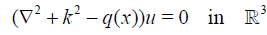 , (1)
, (1)
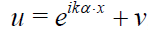 , (2)
, (2)
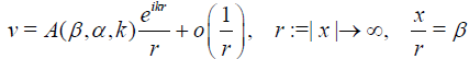 (3)
(3)
where α, β ϵ S2 are the directions of the incident wave and scattered wave correspondingly, S2 is the unit sphere k2 > 0 is energy, k > 0 is a constant, A(β, α, k) is the scattering amplitude (scattering data), which can be measured, and q(x) ϵ Q, where Q is a set of C1-smooth real-valued compactly supported functions, q = 0 for maxj |x| ≥ R, R > 0 is a constant. By D the support of q is denoted.
The direct scattering problem (1) - (3) has a unique solution [1].
Consider now the inverse scattering problem
Find the potential q(x) ϵ Q from the scattering data A(β, α, k). The uniqueness of the inverse scattering problem with fixedenergy data (k = k0 > 0 is fixed) is proved by Ramm [1]: q(x) ϵ Q is uniquely determined by the scattering data A(β, α, k0) for a fixed k = k0 > 0 and all α, β ϵ S2. Ramm also gave a method for solving the inverse scattering problem with fixed-energy data and obtained an error estimate for the solution for exact data and also for noisy data [1], Chapter 5.
In this paper, we give a numerical implementation of the method proposed by A. G. Ramm, for solving the inverse scattering problem with non-over-determined data, that is, finding q(x) ϵ Q from the scattering data A(β, k) := A(β, α0, k) for a fixed α0 ϵ S2, all β ϵ S2 and all k ϵ (a, b), 0 ≤ a < b. The basic uniqueness theorem for this problem is proved, see also [2-7]. In Section 2, the idea of this numerical method is described. This idea and the method described in Section 2 belong to A. G. Ramm. In Section 3, the DSM algorithm used to solve ill-posed linear system is described. In Section 4, the numerical procedure is presented and in Section 5, some examples of the numerical inversion are given.
The essential novel features of this inversion method are:
• The data are non-over-determined. So these are minimal scattering data that allow one to uniquely recover the potential.
• The inverse scattering problem is highly non-linear. Nevertheless, our method reduces the inversion to stable solution of linear algebraic system (8).
• The numerical difficulty comes from the fact that system (8) is highly ill-conditioned.
Inversion method
Let q ϵ Q. The unique solution to (1) - (3) solves the integral equation:
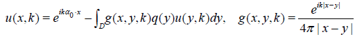 (4)
(4)
k > 0 is a constant, α0 ϵ S2 is fixed. This equation is uniquely solvable for u under our assumptions on q. Let h(x, k) = q(x)u(x, k). Then (4) implies
 .(5)
.(5)
Equations (3) and (4) yield the exact formula for the scattering amplitude:
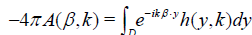 . (6)
. (6)
From equation (5) one derives the formula for q(x) if h(k, x) is found:
 . (7)
. (7)
The idea of our inversion method
By the uniqueness theorem from [6], equation (6) has a unique solution h(x, k). Solve numerically equation (6) for h(x, k). To do this, discretize (6) and get a linear algebraic system for hpm:= h(yp, km). If hpm are found, then q(xp) are found by formula (7), see also formula (9) below.
Let us partition D into P small cubes with volume Δp, 1 ≤ p ≤ P. Let yp be any point inside the small cube Δp. Choose P different numbers km ϵ (a, b), 1 ≤ m ≤ P, and P different vectors βj ϵ S2, 1 ≤ j ≤ P. Then discretize (6) and get a linear algebraic system for finding hpm:
 . (8)
. (8)
Where hpm:= h(yp, km). Solve the linear algebraic system (8) numerically, then use equation (7) to find the values of the unknown potential q(xp):
 (9)
(9)
Remark 1: Note that the right hand side of (9) should not depend on m or j. This independence is an important requirement in the numerical solution of our inverse scattering problem, a compatibility condition for the data. This requirement is automatically satisfied for the limiting integral equation (6), see formula (7).
The values of q(yp) essentially determine the unknown potential q(x) if P is large and q is continuous. The potential q is unique by the uniqueness theorem in [6].
Note that one can choose βj and km so that the determinant of the system (8) is not equal to zero [7], so that the system (8) is uniquely solvable, but the numerical difficulty is unavoidable: the system (8) is very ill-conditioned because it comes from an integral equation (6) of the first kind with an analytic kernel. We use the dynamical system method (DSM) from [2] to solve stably the ill-conditioned system (8).
Dynamical System Method (DSM)
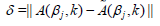
Equation (8) with noisy data is a linear algebraic system of the form
Muδ = fδ (10)
where M is the matrix of the size P × P and fδ is the noisy data, that is, the noisy values of -4πA(βj, km) in equation (8), || fδ - f || = δ for a fixed m and 1 ≤ j ≤ P. To solve this ill-posed system we use the Dynamical Systems Method (DSM) from [2]:
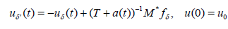 (11)
(11)
where T := M *M, M* is the adjoint matrix and a(t) > 0 is a nonincreasing function such that a(t) → 0 as t → ∞. Equation (11) has a unique solution
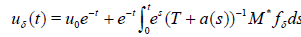 (12)
(12)
To use the DSM method, we need to choose a(t) and find a
stopping time tδ so that uδ(tδ) approximates the solution of Au =
f, so that lim δ → 0 ||uδ - u|| = 0, where the norm is in  .
.
Choice of a(t) and tδ:
In [2], necessary conditions for a(t) are: a(t) is a nonincreasing
function and limt →∞ a(t)=0 . In our experiments, we choose  . Consider a step function ã(t) approximating a(t) :
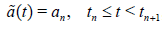 , (13)
where an = a(tn) and we choose tn such that tn+1 - tn = hn, hn = qn, q = 2. From equation (12), one computes un = u(tn) by:
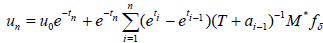 . (14)
and one gets an iterative method to solve (12):
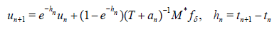 . (15)
To choose tδ, we use a relaxed discrepancy principle [2]:
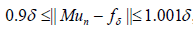 (16)
(16)
where the norm is the vector norm:  . One stops the iterative method (15) when condition (16) is
satisfied.
. One stops the iterative method (15) when condition (16) is
satisfied.
Numerical Procedure and Results
In practice, one can measure the noisy scattering data experimentally. For our numerical experiments, we need to construct the noisy scattering data A(βj, km).
Constructing noisy scattering data
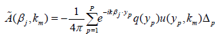
Given a potential q(x), let us first construct the exact scattering data Ã(βj, km). We partition D into P small cubes and discretize equation (4) to get
 . (17)
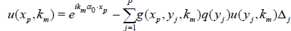
One solves this linear system for u(xp, km) assuming that q(x) is known. Then the exact scattering data are calculated by the following formula:
 . (18)
Then one can randomly perturb each Ã(βj, km), 1≤ j ≤ P by = const > 0 to get the noisy scattering data A(βj, km) = Ã(βj, km)
± where the plus or minus sign is randomly choosen. Then
= const > 0 to get the noisy scattering data A(βj, km) = Ã(βj, km)
± where the plus or minus sign is randomly choosen. Then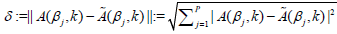 , for a fixed k is
the noise level of the data in equation (10).
, for a fixed k is
the noise level of the data in equation (10).
Numerical procedure
The following steps are implemented in each experiment:
• Choose D, α0, P, q(x), km, and .
• Use (18) to find the exact scattering data Ã(βj, km), 1≤ j ≤ P. Try different values of km so that the determinant of the system in (8) is not zero. Let k be the found value of km.
• Use the procedure in Section 4.1 to get the noisy scattering data A(βj, k), 1≤ j ≤ P.
• Solve the linear algebraic system (8) to get hpm = h(yp, km). Here we use the DSM method in Section 3 with the noise:
 .
.
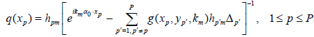
• Calculate the potential  by formula (9):
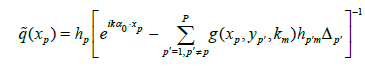 , 1 ≤ p ≤ P
See Remark 1 below formula (9).
• Find the relative error of the estimate of the potential:
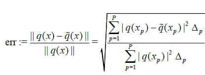 . (19)
Numerical Results
In these experiments, we choose D to be the unit cube centered at the origin, with sides parallel to coordinate planes, P = 1000, α0 = (1, 0, 0), and 50 ≤ km ≤ 100 is chosen so that the determinant of the system in (8) is not zero. The condition number of A is ̴1013.
In the following graphs, the x-axis is the index of the collocation points (this index varies from 1 to 1000) and the y-axis is the value of the potential.
Constant potential with compact support
The inverse scattering problem with constant in D potential is used to test our inversion method. In this experiment, we take q(x) = 10. The results are obtained as in Table 1 and Figure 1.

Figure 1: Constructed potential vs original constant potential q(x) =10 when = 0.01.
| Constant Potential q(x) = 10 | ||
|---|---|---|
| Â |
 |
 Relative Error |
| .04 | Â 0.4348 | Â 0.0566 |
| .02 | Â 0.2174 | Â 0.0037 |
| .01 | Â 0.1087 | Â 0.00065 |
Table 1: Numerical results for constant potential.
Potential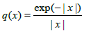
In this experiment, we take . The results are
obtained as in Table 2 and Figure 2.
Figure 2: Constructed potential vs original potential when = 0.01.
| Potential |
||
|---|---|---|
| Â |
  |
 Relative Error |
| .04 | Â 0.0806 | Â 0.1284 |
| .02 | Â 0.0403 | Â 0.0547 |
| .01 | Â 0.0201 | Â 0.0367 |
Table 2: Numerical results for the potential
Conclusion
In this paper, a numerical method is given for solving the inverse scattering problem with non-over-determined scattering data and the numerical results are presented.
References
- Ramm AG.Inverse problems, Springer, New York. 2005;2:1.
- Ramm AG. Dynamical systems method for solving operator equations, Elsevier, Amsterdam. 2007.
- Ramm AG. Inverse scattering with non-over-determined data. Phys Lett A. 2009;2988-91.
- Ramm AG. Uniqueness theorem for inverse scattering problem with non-overdetermined data.J Phys. A. 2010;2:1.
- Ramm AG. Uniqueness of the solution to inverse scattering problem with back-scattering data. Eurasian Math J. 2010;97-111.
- Ramm AG. Uniqueness of the solution to inverse scattering problem with scattering data at a fixed direction of the incident wave. J Math Phys. 2011.
- Ramm AG. A numerical method for solving 3D inverse scattering problem with non-over-determined data. J Pure Appl Math. 2017;1-3.