Research Article - Biomedical Research (2017) Volume 28, Issue 7
Optimized energy aware scheduling to minimize makespan in distributed systems
Rajkumar K1* and Swaminathan P2
1Department of Computer Science and Engineering, School of Computing, SASTRA University, Thanjavur, Tamil Nadu, India
2Dean/School of Engineering, VELS University, Pallavaram, Chennai, Tamil Nadu, India
- *Corresponding Author:
- Rajkumar K
Department of Computer Science and Engineering
School of Computing, SASTRA University
Tamil Nadu, India
Accepted date: November 22, 2016
Abstract
In the present world of large distributed systems and energy shortages, energy efficiency has become mandatory. One way to achieve this is by proper scheduling of tasks in a system of connected and dissimilar machines to minimize the energy consumption. Also, Jobs have to be scheduled properly to different systems in order to achieve maximum utilization of machines. “Makespan” has been the standard optimization criteria used in scheduling algorithms. Makespan is the time elapsed until all jobs scheduled are completely processed. A scheduling algorithm must look to minimize the makespan while satisfying the precedence constraints between the tasks. Though the problem is NP-hard, many algorithms have been proposed. There are algorithms proposed to reduce the energy consumption for uni-machine systems and sequential tasks. Our algorithm tries to reduce the overall energy consumption of a schedule in parallel and distributed systems by minimizing the idle state times of machines and thereby, keeping the makespan as low as possible. Our algorithm is more practical and executes much faster compared to the previous works on energy-aware scheduling.
Keywords
Makespan, Optimization criteria, Precedence constraints, NP-hard, Distributed systems, Idle state time, Energy-aware scheduling.
Introduction
In the modern world, from the perspective of sustainability, there is a growing need for energy efficient scheduling of distributed systems. Much less work has been done on energy aware scheduling and the topic needs more research to be done. Proper scheduling of various tasks on heterogeneous machines can achieve efficiency but scheduling a parallel program on a simplest case of two machine system is itself an NP-complete problem and hence, finding optimal schedules of various dependent and parallel tasks on a number of machines is a very challenging open problem.
Background
Existing approximate solutions using genetic algorithm and cellular automata work on exponential search space and have huge scheduling overheads [1]. Though they seem to be successful in finding near optimal schedules, their execution times are so high that they become useless as the number of tasks and machines increases, increasing the search space exponentially. On the other hand, simple heuristics based techniques execute much faster but often result in a sub optimal solution. Thus, there is a need for a relatively fast algorithm which would also give better schedules. As the number of machines increases, the time for which each machine remains idle also increases. In that case, the total power consumption of a schedule is largely dependent on the idle state power consumptions of each machine. Increasing the utilization of each machine reduces the overall idle state power consumption of the system and hence the total energy of schedule. Also, increasing the utilization means more packed scheduling and hence, lesser makespan. Thus, minimizing makespan and energy complement each other as the number of machines increases. The existing algorithms on energy aware scheduling [1] have assumed the task weight (execution time of a task) to be the same on all the connected machines which is not the case in real world heterogeneous distributed systems [2-4].
Our Work
The objective of our work is to develop a relatively fast algorithm which would take in the configuration of machines, the dependencies among tasks and power specification of machines as inputs and produce a near optimal schedule which minimizes both makespan and the total energy consumption of the schedule. The algorithm must also be more practical and model the real world heterogeneous distributed systems well. Our algorithm optimizes the program graph level-wise, recursively with a backtracking implementation. Each level is separately optimized and the final near optimal schedule is obtained by combining the level-wise optimized sub-schedules. Thus, the problem is split into a number of sub problems and the final solution is obtained by combining the optimal sub solutions. A formal definition of the scheduling problem and our proposed algorithm is explained in Section II. The results obtained by simulating our algorithm on standard program graphs are presented in Section III. The conclusion and the scope for future work are discussed in Section IV.
Energy Efficient Makespan Scheduling (EEM Scheduling)
The system model we have used is the same as proposed by Agrawal et al. [1] with a slight modification in the program graph so that it models the real world heterogeneous distributed systems well. The algorithm takes in a system graph, a program graph and power specifications of machines and maps each task in the program graph to a machine in the system graph such that the total energy of the schedule and the makespan are both kept low.
System model
The system model consists of a system graph, power specifications of machines and a program graph [1].
System graph: It is an unweighted undirected graph describing the connections between individual machines of the system. The cardinality Nm is the number of machines. In our simulations, we have assumed a fully connected mesh topology with Nm=2, 4, 8.
Program graph: It describes each task and dependencies among different tasks. Each node represents a task and the edges represent the dependencies among various tasks. Each node is associated with a list of weights. The weight w (i, j) of node i is the execution time of task i on machine j. The edge weight represents the transfer cost which is the cost of communication when the two nodes connected by the edge are scheduled in different machines. Figure 1 shows an example modified program graph which models the real world distributed systems well.

Figure 1: An example program graph: Weight lists denote execution costs of various tasks on various machines. Edge weights denote transfer costs and direction of edges denote precedence constraints.
Power specifications: Each machine’s power specification is represented by its active state and idle state power consumptions (Table 1).
| Symbol | Meaning |
|---|---|
| μ (Cu) | Power consumption of machine Cu in working state |
| kμ (Cu) | Power consumption of machine Cu in idle state. 0<=k<=1 |
| τc (Cu) | Time for which machine Cu remains in working state |
| τi (Cu) | Time for which machine Cu remains in idle state |
Table 1: Power consumption specification [1].
Brute force solution
Let the number of tasks be Nt. A simple brute force solution for finding the optimal schedule would be to try all possible combinations of tasks on all machines. In that case, each task might be scheduled in any of the Nm machines. This algorithm is exponential with respect to both number of tasks and number of machines. The complexity of the algorithm is O (NmNt). This is clearly not practical to implement and use in any real world industry. However, this solution can be optimized greatly which would result in a very near optimal solution and also have practical running times [5,6].
Proposed technique and complexity
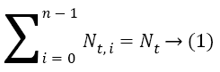
Our algorithm splits the scheduling problem into various sub problems, each sub-problem being finding an optimal schedule of tasks in a single level in the program graph. Since tasks within a single level can be effectively parallelized and tasks in different levels have dependencies among them and have to be scheduled one after the other, it is a very reasonable approximation to find optimal schedules of each level separately and then combine the optimal sub-schedules which would result in a global near optimal solution. Let the number of tasks in level i be Nt, i and the number of levels be n. We have,
Clearly,
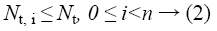

Hence, the complexity of level wise optimized brute force solution would be  which is way better than O (NmNt). Clearly, this is a better solution compared to the normal brute force but this still is impractical when tasks count in a single level increases beyond a certain number. Though there may be a number of tasks in a single level, we cannot have more than Nm tasks executing at the same time since we have only Nm machines. In that case, we can split the tasks in a single level into subsets, each subset having at most Nm tasks and schedule each subset optimally using brute force (i.e. when we have 12 tasks and 4 machines, at any point in time we can only have at most 4 tasks executing in parallel. Thus the 12 tasks can be split into 3 sets of 4 tasks each and each set can be scheduled optimally using brute force). Thus, we have sub-problems within a sub-problem. This is the technique that we propose.
The complexity of scheduling each level i in the proposed approach is less than or equal to O (Nt, i/Nm× NmNm), 0 ≤ i<n. Hence the complexity of the complete algorithm is always less than or equal to O (Nt/Nm×NmNm). We could clearly see that the complexity of the proposed algorithm is no longer exponential with respect to the number of tasks. Considering the fact that earlier works on energy efficient or minimum makespan task scheduling in heterogeneous distributed systems have considered systems with a maximum of 8 machines, our algorithm finds a near optimal schedule in less than 10 seconds which is extremely faster compared to the existing algorithms.
The energy consumption of the resultant schedule is calculated as follows [1].
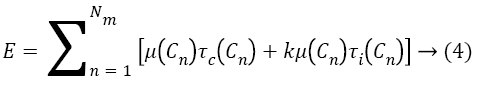
In order to minimize E, we would have to minimize τi (Cn) μ (Cn) and kμ (Cn) are fixed for a given set of machines. Also, the sum of execution times of all the tasks does not vary significantly on increasing the number of machines. Hence, the only parameter that significantly varies as the number of machines increases is the time for which each machine remains idle. If we can minimize this parameter, we would obtain an energy efficient schedule. The utilization of each machine is obtained from the formula [7].
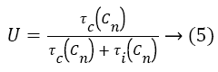
Clearly, minimizing idle times of machines (τi (Cn)) increases the utilization. As the utilization of each machine is improved, we get more packed scheduling and thus end up with reduced makespans [1,8]. Thus, minimizing total energy consumption and minimizing makespan complement each other.
Dynamic programming optimization
Within each level, nodes have to be considered in some order for scheduling by the brute force logic [6]. This order is determined by the total number of tasks in the higher levels which are dependent on the tasks in the lower levels. Scheduling earlier a task which has more number of dependent tasks minimizes the makespan, as those dependent tasks can also be now scheduled earlier. Hence, nodes in each level are ranked based on the total number of outgoing edges from each node and its successor nodes recursively. Let R (i, j) be the rank of jth node in ith level and s be the number of immediate successors of that node. We have,
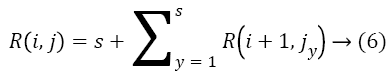
Where R (i+1, jy) is the rank of yth successor of jth node in level i. We have solved this recurrence using dynamic programming. The nodes in the bottom most level of the program graph have no outgoing edges and hence their ranks would be 0. Traversing the graph from the bottom most level to the root level, we assign ranks to each node in each level as per the recurrence relation given. We thus have each level sorted, passing which to the brute force algorithm results in better sub schedule and overall near optimal solution [2,9].
The criteria used for determining the best sub schedule by the brute force algorithm can either be time or energy. Surprisingly, results of simulating our algorithm on standard graphs like g18, g40, tree15 and guass18 with minimum time as the criterion for choosing the best sub schedule in each level, resulted in overall schedules which had better energy values than the overall schedules that were obtained using minimum energy as the criterion for choosing best sub schedules in each level. This supports our claim that minimizing makespan by minimizing the idle state times of each machine, reduces the overall energy consumption. Thus minimizing time and energy complement each other [4,10].
Algorithm

Algorithm 1: Algorithm for CA+GA.
Algorithm 2: The proposed algorithm
Our algorithm uses the user defined classes as described in Table 2.
| Class | Data members | |
|---|---|---|
| Variable | Type | |
| Task | name | Integer |
| weight_list | ArrayList | |
| predecessor | ArrayList | |
| Machine | name | Integer |
| idle_pwr | Float | |
| active_pwr | Float | |
| Task Schedule | task | Task |
| machine | Machine | |
| start_time | Integer | |
| end_time | Integer | |
Table 2: Classes used by EEM scheduling algorithm.
Other variables that are used by the algorithm are as follows
• Task_obj, which is an array list of objects of Task class. It stores the details of each task.
• Machine_obj, which is an array list of objects of Machine class. It stores the details of each machine.
• Transfer_cost, which is a two dimensional adjacency matrix of integer type. transfer_cost [i] [j] is equal to the communication cost if tasks i and j are scheduled in different machines. It is equal to -1, if there is no edge between tasks i and j.
• Schedule_graph, which is a two dimensional array list of objects of Task Schedule class. It stores the details of where and when each task is scheduled. schedule_graph [i] gives the schedule of ith machine.
• Sched, which is an array list of objects of TaskScheduleclass. It stores the details of how each task is scheduled, their start times, end times and machines in which they are scheduled.
• Levels, which is a two dimensional array list of integers storing the individual levels in the program graph.
• Total_energy, which is a float variable storing the total energy consumption of the best schedule.
The steps involved in the algorithm are as follows.
1. Get the system graph, program graph and power specification as input
2. Populate task_obj, machine_obj and transfer_cost adjacency matrix
3. Split the program graph level-wise and store the individual levels in levels
4. Sort the nodes in each level based on the rank (number of outgoing links from each node and its successor nodes recursively). We use dynamic programming to simplify this step.
5. Initialize schedule_graph and sched objects
6. For every level ‘i ‘do,
7. Split the tasks in level ‘i’ to sets of at most Nm elements and call schedule_level () on each set.
8. Update schedule_graph
9. Update sched
10. Calculate total_energy and print it
11. Print schedule_graph
Function schedule_level () tries all combinations of tasks in the specified set that is passed as a parameter, and returns the best schedule with minimum running time [1,11,12].
Results
Our algorithm was tested on standard program graphs like tree15, g18, guass18 and g40 with Nm=2, 4, 8 (Tables 3-5). Though our algorithm allows for any number of machines with different working and idle state power consumptions, generally, existing algorithms on scheduling consider lesser than 8 machines. So, we have shown here the results for 2, 4 and 8 machine systems so that they are easily compared with the existing algorithms’ results.
| Graph | Active state energy | Idle state energy | Total energy consumption | Makespan | Running time (in seconds) |
|---|---|---|---|---|---|
| tree15 | 15.0 | 17.0 | 32.0 | 8 | 0.147 |
| g18 | 86.0 | 22.0 | 108.0 | 27 | 0.160 |
| guass18 | 60.0 | 148.0 | 208.0 | 52 | 0.149 |
| g40 | 160.0 | 24.0 | 184.0 | 46 | 0.173 |
Table 3: Makespan and energy comparison, with Nm=4, k=1.
| Graph | Active state energy | Idle state energy | Total energy consumption | Makespan | Running time (in seconds) |
|---|---|---|---|---|---|
| tree15 | 15.0 | 41.0 | 56.0 | 7 | 2.382 |
| g18 | 86.0 | 106.0 | 192.0 | 24 | 2.346 |
| guass18 | 60.0 | 356.0 | 416.0 | 52 | 0.377 |
| g40 | 160.0 | 88.0 | 248.0 | 31 | 9.236 |
Table 4: Makespan and energy comparison, with Nm=8, k=1.
| Graph | Active state energy | Idle state energy | Total energy consumption | Makespan | Running time (in seconds) |
|---|---|---|---|---|---|
| tree15 | 15.0 | 78.0 | 93.0 | 5 | 4.281 |
| g18 | 86.0 | 210.0 | 296.0 | 20 | 3.831 |
| guass18 | 60.0 | 550.0 | 610.0 | 48 | 0.934 |
| g40 | 160.0 | 103.0 | 263.0 | 24 | 9.842 |
Table 5: Makespan and energy comparison, with Nm=16, k=1.
The tree15 graph displayed in Figure 2 is a binary tree with all communication and execution costs equalling unity. The g18 graph is shown in Figure 3. Though our algorithm allows for different execution costs on different machines for the same task, for the purpose of comparing our results with that of the previous works, our algorithm was simulated on the same program graphs which were used by Agrawal et al. [1,13].

Figure 2: Architecture of CA+GA.

Figure 3: Tree15Program Graph: All communication and execution costs are unity.
The guass18 graph is displayed in Figure 4 with the specified execution and communication costs. The g40 graph is shown in Figure 5 with all communication and execution costs equalling unity.

Figure 4: G18 Program Graph: All communication costs equal unity.

Figure 5: Guass18 Program Graph: All communication and execution costs are as specified.
Figure 6 compares the total energy of the schedules produced by the CA+GA algorithm proposed by Agrawal et al. [1] and EEM scheduling that we have proposed. Clearly, EEM results in better schedules in terms of energy on all the standard graphs. Figure 7 is a comparison of the time taken by both these algorithms to produce a near optimal schedule. The exponential dependency of the CA+GA algorithm on both the number of machines and the number of tasks results in huge execution times whereas, EEM scheduling algorithm’s running time does not have an exponential dependence on the number of tasks to be scheduled. Since the number of machines is constant, we could see an almost constant running time of EEM algorithm on all the standard graphs that we tested our algorithm on. Same is the case when Nm=4. Figure 8 shows the comparison of the makespan of the final schedules produced by CA+GA (i.e. in Figure 2) and EEM scheduling. Our algorithm produces much better results on three of the four graphs.

Figure 6: g40 Program Graph: All communication and execution costs are unity.

Figure 7: Energy comparison of existing and proposed algorithms with Nm=8, k=1.

Figure 8: Running time comparison of existing and proposed algorithms with Nm=8.
An analysis of the guass18 program graph makes it clear that unlike other graphs, in guass18, we have nodes in higher levels having greater number of dependent nodes than the ones at the lower levels (i.e. Figure 4, node 11 has more number of outgoing edges than node 5). Also, the higher transfer costs associated, restricts the brute force logic from producing locally sub optimal parallel schedules which might result in globally near optimal solution. To overcome this, we tried modifying our algorithm so that, instead of considering nodes level-wise for scheduling, it would rank all the nodes based on the total number of nodes at the higher levels that are dependent on them. It then splits the nodes into Nt/Nm sets, each of which is sequentially scheduled. But doing that, we failed to schedule parallel processes in the same level efficiently, when we have higher ranked nodes in the higher levels. Since, only nodes within a level can be parallelized and we lose this parallelism by modifying the algorithm, the results of the modified algorithm was not better than the proposed algorithm. However, the small increase in makespan of the schedule produced by the proposed EEM algorithm in the case of guass18 graph is more than compensated by the huge running time of the CA+GA algorithm (Figure 9) to find the schedule which is only a bit better than our solution [1,14].

Figure 9: Makespan comparison of existing and proposed algorithms.
Conclusion
As proposed, we have been successful in generating near optimal energy-efficient and minimum makespan schedules for tasks on heterogeneous distributed systems with varying power consumptions and task execution times. From the simulation results, it is clear that our algorithm runs extremely faster and generates much better schedules compared to the existing systems. When the execution time of tasks on different machines vary, our algorithm concentrates on minimizing the idle power consumption and hence the makespan, which in turn reduces the total energy consumption (Figure 10) [15]. However, when more than one sub-schedule satisfy the minimum time or energy criterion of the brute force logic, our algorithm always chooses the first such sub-schedule that it encountered, whereas choosing the other sub-schedules might result in a better overall schedule. We could work on ranking the equally good sub-schedules in each level so that the highest ranked schedule would result in a better overall schedule.
Also, the other drawback of the algorithm on graphs like guass18, as explained in Section III requires much deeper analysis and understanding of the graphs by the algorithm. Developing a generic algorithm which would dynamically schedule different graphs differently so that, the algorithm returns a near optimal solution on all types of graphs can be seen as the possible next step.

Figure 10: Energy consumption for graph g40.
References
- Agrawal P, Rao S. Energy-aware scheduling of distributed systems, automation science and engineering. IEEE Trans 2014; 11: 1163,1175.
- Santhi B, Thambidurai P. Energy efficient real-time scheduling in distributed systems. Int J Comp Sci Iss 2010; 7: 35-42.
- Dawei L, Jie W. Minimizing energy consumption for frame-based tasks on heterogeneous multiprocessor platforms, parallel and distributed systems. IEEE Transactions 2015; 26: 810,823.
- Keqin L. Power allocation and task scheduling on multiprocessor computers with energy and time constraints. Energy-Efficient Distributed Computing Systems John Wiley Inc. Hoboken New Jersey USA (1st edn.) 2012.
- Liu J, Chou P, Bagherzadeh N, Kurdahi F. Power-aware scheduling under timing constraints for mission-critical embedded systems. Proc Design Autom Conf 2001; 840-845.
- Garey M, Johnson D. Computers and intractability: A guide to the theory of np- completeness. WH Freeman co. New York USA 1979.
- Jian JH, Man L, Dakai Z, Laurence TY. Contention-aware energy management scheme for NOC-based multicore real-time systems, parallel and distributed systems. IEEE Trans 2015; 26: 691,701.
- Zomaya AY, Lee YC. Energy-efficient distributed computing systems. New York USA Wiley 2012.
- Sheikh HF, Tan H, Ahmad I, Ranka S, Bv P. Energy- and performance-aware scheduling of tasks on parallel and distributed systems. ACM J Emerg Technol Comp Sys 2012; 8.
- Kenli L, Xiaoyong T, Keqin L. Energy-efficient stochastic task scheduling on heterogeneous computing systems, parallel and distributed systems. IEEE Trans 2014; 25: 691,701.
- Lee YC, Zomaya AY. Energy conscious scheduling for distributed computing systems under different operating conditions. IEEE Trans Parallel Distrib Sys 2011; 22: 1374-1381.
- Metin T, Hasan S, Ibrahim K. Distributed construction and maintenance of bandwidth and energy efficient bluetooth scatternets,parallel and distributed systems. IEEE Trans 2006; 17: 963-974.
- Garey M, Johnson D. Computers and intractability: A guide to the theory of NP-completeness. New York NY USA WH Freeman 1979.
- Li Y, Liu Y, Qian D. A heuristic energy-aware scheduling algorithm for heterogeneous clusters. Proc 15th Int Conf Parallel Distrib Sys 2009; 407-413.
- Artigues C, Lopez P, Hait A. Scheduling under energy constraints. Int Conf Ind Eng Syst Manage 2009.