Research Paper - Journal of Applied Mathematics and Statistical Applications (2018) Volume 1, Issue 2

On the asymptotic behavior of the deficiency of some statistical estimators based on samples with random sizes

*Corresponding Author:

V.E. Bening
Faculty of Computational Mathematics and Cybernetics Lomonosov Moscow State University Russia
Tel: +7 495 939-31-21
E-mail: bening@yandex.ru

Accepted date: 26, 2018, 2018;

Citation: Bening VE. On the asymptotic behavior of the deficiency of some statistical estimators based on samples with random sizes.. J Appl Math Statist Appl. 2018;2(1):32-41.

Abstract

Due to the stochastic character of the intensities of information flows in high performance information systems, the size of data available for the statistical analysis can be often regarded as random. The purpose of this paper is to present some means for the comparison of the quality of estimators constructed from samples with random sizes with that of estimators constructed from samples with non-random sizes. As this means it is proposed to use the deficiency. It can be an illustrative characteristic of a possible loss of the accuracy of statistical inference if a random-size-sample is erroneously regarded as a sample with non-random size. It is heuristically shown that if the asymptotic distribution of the sample size normalized by its expectation is not degenerate, then the deficiency of a statistic constructed from a sample with random size whose expectation equals n with respect to the same statistic constructed as if the sample size was non-random and equal to n, grows almost linearly as n grows. A non-trivial behavior of the deficiency is possible only if the random sample size is asymptotically degenerate. This is the case considered in the paper where the deficiencies of statistics constructed from samples whose sizes have the Poisson, binomial and special three-point distributions, respectively, are considered. Some basic results dealing with some properties of estimators based on the samples with random sizes are also presented.

Keywords

Estimator, Risk function, Deficiency, Asymptotic deficiency, Sample with random size, Asymptotic expansions, Poisson distribution, Binomial distribution, Three-point distribution.

Introduction

Motivation for the consideration of statistics constructed from samples with random sizes

In most cases related to the analysis of experimental data, the number of random factors which influence observed objects is random and changes from one observation to anorher. Due to the stochastic character of the intensities of information flows in high performance information systems, the size of data available for the statistical analysis can be often regarded as random. In classical problems of mathematical statistics, the size of the available sample, i. e., the number of available observations, is traditionally assumed to be deterministic. In the asymptotic settings it plays the role of infinitely increasing known parameter. At the same time, in practice very often the data to be analyzed is collected or registered during a certain period of time and the flow of informative events each of which brings a next observation forms a random point process. Therefore, the number of available observations is unknown till the end of the process of their registration and also must be treated as a (random) observation. For example, this is so in insurance statistics where during different accounting periods different numbers of insurance events (insurance claims or insurance contracts) occur and in high performance information systems where due to the stochastic character of the intensities of information flows, the size of data available for the statistical analysis can be often regarded as random. Say, the statistical algorithms applied in high-frequency financial applications must take into consideration that the number of events in a limit order book during a time unit essentially depends on the intensity of order flows. Moreover, contemporary statistical procedures of insurance and financial mathematics do take this circumstance into consideration as one of possible ways of dealing with heavy tails. However, in other fields such as medical statistics or quality control this approach has not become conventional yet although the number of patients with a certain disease varies from month to month due to seasonal factors or from year to year due to some epidemic reasons and the number of failed items varies from lot to lot. In these cases the number of available observations as well as the observations themselves are unknown beforehand and should be treated as random to avoid underestimation of risks or error probabilities.

In asymptotic settings, statistics constructed from samples with random sizes are special cases of random sequences with random indices. The randomness of indices usually leads to that the limit distributions for the corresponding random sequences are heavy-tailed even in the situations where the distributions of non-randomly indexed random sequences are asymptotically normal [1-3]. For example, if a statistic which is asymptotically normal in the traditional sense, is constructed on the basis of a sample with random size having negative binomial distribution, then instead of the expected normal law, the Student distribution with power-type decreasing heavy tails appears as an asymptotic law for this statistic [1,4].

At the same time, according to the conventional logics of the statistical analysis, the distributions of the statistics (estimators, tests, etc.) to be used for the statistical inference should be known before the actual sample is observed in order to calculate critical values or thresholds. As a rule, asymptotic approximations by limit distributions of statistics are used instead of the exact distributions because the former are considerably easier computable than the latter. As this is so, in limit theorems of probability theory and mathematical statistics the centering and normalization of random variables are used to obtain non-trivial asymptotic distributions. It should be especially noted that to obtain reasonable approximation to the distribution of the basic random variables, both centering and normalizing values should be non-random. Otherwise the approximate distribution becomes random itself and, say, the problem of evaluation of quantiles required for the calculation of critical values or confidence intervals becomes senseless.

Throughout the paper we use conventional notation: is the set of real numbers, is the set of natural numbers, h(n) ~ f(n), n → ∞ if and only if . The symbols ,⇒ and denote the coincidence of distributions, convergence in distribution and the end of the proof, respectively.

Consider a family of probability measures each of which is defined on a measurable space (Ω,) . Consider a sequence of random variables (r.v.’s) X₁, X₂,… defined on a measurable space (Ω,) . Everywhere in what follows consider the random variables X₁, X₂,… to be independent and identically distributed (i.i.d) with common distribution P_θ . Let N₁, N₂,… be a sequence of nonnegative integer random variables with common distribution P defined on the same measurable space so that for each n ≥ 1 the random variable N_n is independent of the sequence X₁, X₂,… with respect to any measure P_θ from ρ . A random sequence N₁, N₂,… ( Ni with distribution P, i = 1, 2,…) is said to be infinitely increasing (N_n → ∞) in probability P, if P (N_n≤ M) → 0 as n → ∞ for any M ϵ (0, ∞). For n ≥ 1, let T_n = T_n (X₁,…, X_n) be a statistic, that is, a measurable function of the r.v.’s X₁,…, Xn. For each n ≥ 1 define the r.v. TN_n by letting:

for every elementary outcome ω ϵ Ω. Assume that for each θ ϵ Θ there exists:

where , is the expectation w.r.t. distribution , of T_n . We will say that the statistic T_n is asymptotically normal,

,

if

for each θ ϵ Θ.

The following statement describes the change of the limit law of an asymptotically normal statistic when the sample size is replaced by a r.v. (Theorem 3.3.2) [5].

Lemma 1.1. Assume that N_n → ∞ in probability P as n → ∞. Let the statistic T_n be asymptotically normal in the sense of

(1.1) . Then a distribution function F(x) such that

,

exists if and only if there exists a distribution function Q(x) satisfying the conditions Q(0) = 0 ,

.

The concept of deficiency

Before turning to the general case of statistics constructed from samples with random size, that is the main aim of the present paper, let us recall the notion of a deficiency of a statistical estimator for the traditional case where the sample size is nonrandom [6].

Suppose that T_n (X₁,…, X_n) and T_n (X₁,…, X_n) are two competing estimators of g(θ), θ ϵ Θ based on n observations X₁,…, X_n and let their expected squared errors (risk functions) be denoted by and , respectively. An interesting quantitative comparison can be obtained by taking a viewpoint similar to that of the asymptotic relative efficiency (ARE) of estimators, and asking for the number m(n) of observations needed by estimato T_m(n) (X₁,…, X_m(n)) to match the performance of T_n^* (X₁,…, X_n) (based on n observations). The asymptotic (as n → ∞) comparison of the two estimators involves the comparison of m(n) with n, and this can be carried out in various ways. Although the difference m(n) - n seems to be a very natural quantity to examine, historically the ratio n / m(n) was preferred by almost all authors in view of its simpler behavior. The first general investigation of m(n) - n was carried out by Hodges and Lehmann [5]. They name m(n) - n the deficiency of T_n with respect to T_n^* and denote it as:

Suppose that for n → ∞, the ratio n / m(n) tends to a limit b, the asymptotic relative efficiency of T_n (X₁,…, X_n) with respect to T_n^* (X₁,…, X_n) . If 0 < b< 1, we have d_n ~ (b^-1 - 1) n and further asymptotic information about d_n is not particularly revealing. On the other hand, if b=1, the asymptotic behavior of dn, which may now be varying from o(1) to o(n), does provide important additional information.

If limn _{n →∞}d_n exists, it is called the asymptotic deficiency of T_n with respect to T_n^* and denoted d. At points where no confusion is likely, we shall simply call d the deficiency of T_n with respect to T_n^*.

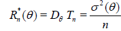
The deficiency of T_n relative to T_n^* will then indicate how many observations one loses by insisting on T_n , and thereby provides a basis for deciding whether or not the price is too high. If the risk functions of these two estimators are:

,

then, by definition, d_n(θ) = d_n = m(n) - n, for each n, may be found from

In order to solve (1.3), m(n) has to be treated as a continuous variable. This can be done in a satisfactory manner by defining R_m(n)( θ) for non-integer m(n) as:

[6].

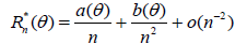
Generally R_n^*(θ) and R_n(θ) are not known exactly and we have to use approximations. Here these are obtained by observing that R_n^*(θ) and R_n(θ) will typically satisfy asymptotic expansions (a.e.) of the form:

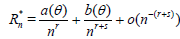, (1.4)

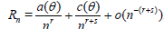, (1.5)

for certain a(θ), b(θ) and c(θ) not depending on n and certain constants r > 0, s > 0. The leading term in both expansions is the same in view of the fact that ARE is equal to one. From (1.2) - (1.5) is now easily follows that [6]

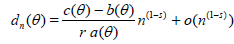. (1.6)

Hence,

. (1.7)

A useful property of deficiencies is the following (transitivity): if a third estimator is given, for which the risk also has an expansion of the form (1.5), the deficiency d of with respect to T_n^* satisfies the relation d = d₁+ d₂, where d₁ is the deficiency of T_n^* with respect to T_n and d₂ is the deficiency of T_n with respect to T_n^*.

The situation where s = 1 seems to be the most interesting one. Hodges and Lehmann [6] demonstrate the use of deficiency in a number of simple examples for which this is the case (for testing problems see also [7-10]).

The purpose and structure of the paper

The purpose of this paper is to present some means for the comparison of the quality of estimators constructed from samples with random sizes with that of estimators constructed from samples with non-random sizes. As this means we propose to use the deficiency. It can be an illustrative characteristic of a possible loss of the accuracy of statistical inference if a randomsize- sample is erroneously regarded as a sample with nonrandom size. The present paper develops the research started [3] and presents a number of applications of the deficiency concept in problems of point estimation in the case when the number of observations is random.

Section 2 contains main results. First, in Section 2.1 we heuristically show that if the d.f. Q(x) in Lemma 1.1 is not degenerate, then the deficiency of a statistic constructed from a sample with random size whose expectation equals n with respect to the same statistic constructed as if the sample size was non-random and equal to n, grows almost linearly as n grows. A non-trivial behavior of the deficiency is possible only if the random sample size is asymptotically degenerate. This is the case considered in Sections 2.3, 2.4 and 2.5 where the deficiencies of statistics constructed from samples whose sizes have the Poisson, binomial and special three-point distributions, respectively, are considered. Section 2.2 contains some preliminary basic results dealing with some properties of estimators based on the samples with random sizes. Sections 3 - 5 contain results concerning deficiencies of asymptotic quantiles.

In this paper we focus on the case where the sample size is independent of the r.v.’s forming the sample. This assumption, first, is made for the sake of simplicity of the methods used to obtain the qualitative results. Second, in many applied problems this assumption does not contradict the essence of the problem. For example, this is so when the data is accumulated within a prescribed time interval (a month, a year, etc.), but the informative events form a stochastic flow. This situation is typical for financial and insurance practice or any other field of activities with accounting periods. Moreover, the independence of X₁, X₂,… is not crucial since basic Lemma 1.1 can be proved without this assumption [5]. Third, most papers considering non-independent sample sizes deal with the case of asymptotically degenerate indexes. This is just the case yielding non-trivial results in the present paper. It seems that using martingale techniques or imposing some concrete conditions on the character of dependence between the sample elements and the sample size, the results of this paper can be extended for the non-independent case.

Deficiencies of Some Estimators Based on the Samples with Random Size

The asymptotic behavior of the deficiency of a statistic constructed from a sample with random size

The interpretation of the deficiency as the number of additional observations required to attain the same quality here needs to be refined since this number becomes random in random-sizesamples problems. In order to circumvent this difficulty assume that the r.v.’s N₁, N₂,… are parameterized by their expectations:

This assumption will enable us, instead of comparing random variables, to compare their easily tractable parameters.

Before we construct the exact formulas for the deficiencies so tractable, we have to make some important heuristic comments concerning the boundedness of the deficiency as a function of the parameter n. By X without any indexes we will denote a r.v. with the standard normal distribution N(0, 1). Let Tn be an asymptotically normal (1.1) (with σ(θ) = 1) statistic constructed from the sample X₁, X₂,…, be (the same) statistic constructed from the random-size-sample . Assume that, , implying , (Theorem 2.1). Denote,

From Lemma 1.1, for n large enough we have the approximate relations:

Where,

and the r.v.’s X and U are independent. Therefore,

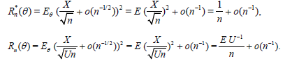
Equating R_n^*(θ) and R_m(n)( θ) we obtain,

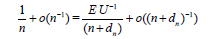
or

Where,

D = E U⁻¹ −1.

So, in general, if EU⁻¹ ≥ 1, then d_n = O(n) . And the only possibility for dn to be o(n) and, in particular, to remain bounded, is the case:

E U⁻¹ =1.

In general, if in addition to the conditions of Lemma 1.1, the family {Nn / n}_{n ≥ 1} is uniformly integrable, then the conditions of Lemma 1.1 and E Nn = n imply that EU =1, so that by the Jensen inequality we have EU⁻¹ ≥ 1 with the equality attainable if and only if

P (U =1) =1.

In other words, for the deficiency d_n to be bounded in n, it is necessary that the sample size N_n should be asymptotically degenerate in the sense that

in probability as n → ∞. This property is inherent in sample sizes with the Poisson, binomial and special three-point distributions considered in the present paper.

It is worth noting that an example of geometrically distributed Nn for which the limit r.v. U as the exponential distribution vividly illustrates the possibility of the deficiency to be unbounded since in this case the Fréchet distribution of the r.v. U-1 has the infinite first moment.

Summarizing the abovesaid we conclude that if the d.f. Q(x) in Lemma 1.1 is not degenerate, then the deficiency of a statistic constructed from a sample with random size whose expectation equals n with respect to the same statistic constructed as if the sample size was non-random and equal to n, grows almost linearly as n grows. A non-trivial behavior of the deficiency is possible only if the random sample size is asymptotically degenerate. This is the case to be considered in the present paper.

Some properties of estimators based on the samples with random sizes

Assume that for each n ≥ 1 the r.v. N_n takes only natural values (i.e., ) and is independent of the sequence X₁, X₂,… Everywhere in what follows the r.v.’s X₁, X₂,… are assumed independent and identically distributed with distribution depending on .

Recall that we assume that,

that is, the expected sample size equals the sample size for the case where it is non-random, that is, the r.v. N_n is parameterized by its expectation n.

Theorem 2.1.

1. If

Then,

.

2 . Let

.

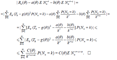
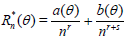
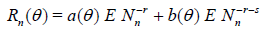
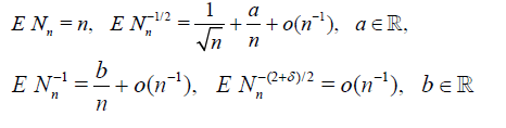
Assume that there exist numbers a(θ), b(θ), C(θ) > 0, α > 0, r > 0 and s > 0 such that

Then,

.

Proof: The desired relations can be easily obtained by the formula of total probability formula. Namely, we obviously have

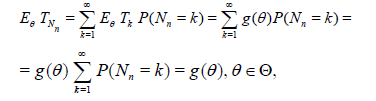
and

Corollary 2.1. Let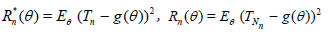

. Assume that there exist numbers a(θ), b(θ), r > 0 and s > 0 such that

.

Then,

.

Consider some examples.

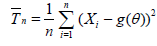
1. Let observations X₁,…, X_n have expectation E_θX₁ = g(θ) and variance D_θX₁= σ²(θ). The customary estimator for g(θ) based on n observation is

.(2.1)

This estimator is unbiased and consistent, and its variance is

. (2.2)

If this estimator is based on the sample with random size, then we have (see Corollary 2.1)

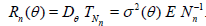(2.3)

2. Now, if g(θ) is given, for σ²(θ) we consider the estimator of the form

. (2.4)

This estimator is unbiased and consistent, and its variance is

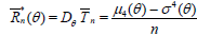, (2.5)

Where, . For this estimator based on a sample with random size we have

. (2.6)

3. In the preceding example suppose that g(θ) is unknown and instead of (2.4) we consider any estimator of the form

, (2.7)

with T_n defined in (2.1). If γ ≠ -1, this estimator is not unbiased but may have a less expected squared error than the unbiased estimator with γ = -1. One easily obtains (3.6) [6].

and hence,

. (2.8)

Using Theorem 2.1 we have

. (2.9)

Deficiencies of some estimators based on samples with random size having the Poisson distribution

When the deficiencies of statistical estimators constructed from samples of random size and the corresponding estimators constructed from samples of non-random size n (under the condition EN_n = n) are evaluated, we actually compare the expected size m(n) of a random sample with n by means of the quantity d_n = m(n) - n and its limit value.

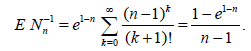
We will now apply the results of Section 2.2 to the three examples. We begin with the case of the Poisson-distributed sample size. Let M_n be the Poisson r.v. with parameter n – 1, n ≥ 2, i.e.

, k=0,1,....

Define the random sample size as N_n = M_n + 1. Then, obviously, EN_n = n and

Expanding the exponent in the Taylor series, we easily obtain that

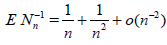. (2.10)

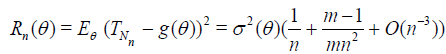
The deficiency of relative to T_n (see (2.1)) is given by (2.2), (2.3), (2.10) and (1.7) with r = s = 1, a(θ) = σ²(θ), b(θ) = 0, c(θ) = σ4(θ), and hence, is equal to

d =1.

Similarly, the deficiency of relative to (see (2.4)) is given by (2.5), (2.6), (2.10) and (1.7) with r = s = 1, a(θ) = c(θ) = μ₄(θ) - σ₄(θ), b(θ) = 0, and hence, is equal to

.

Now consider the third example (see (2.7)). We have

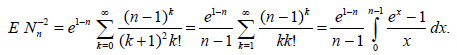
Using the Bernoulli – L’H ˆ o pital principle we obtain

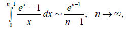
and

. (2.11)

Now the deficiency of with respect to (see (2.7)) is given by (2.8), (2.9), (2.11) and (1.7) with r = s = 1 and hence, is equal to

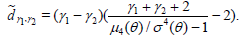
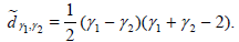
whereas the deficiency of (γ₁) with respect to (γ₂) (see (2.7)) is given by (2.10), (2.11) and (1.7) with r = s = 1 and hence, is equal to

Thus, the classical (0) is better than (-1) , if

,

with the situation reversed, if

.

In particular, if X₁ is normal, then

and

One can therefore save an expected 3 / 2 observations by using the biased estimator (0) . The best value of γ in the normal case is γ = 1 for which and which therefore provides an additional saving 1 / 2 observations.

These examples illustrate the following statement.

Theorem 2.2. Assume that there exist numbers a(θ), b(θ) and k₁, k₂ such that

and

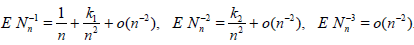
Then the asymptotic deficiency of with respect to T_n is equal to

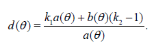
The proof follows from Theorem 2.1, (1.6) and (1.7).

Deficiencies of some estimators based on samples with random size having the binomial distribution

In this Section the results obtained above will be applied to the calculation of the deficiencies of the estimators T_n , , (see (2.1), (2.4) and (2.7)) constructed from samples whose sizes are random and have the binomial distribution.

Using the definition of the binomial distribution we directly obtain the following statement.

Lemma 2.1. Let the r.v. B_n have the binomial distribution with the parameters m(n - 1), n ≥ 2 and p = 1 / m, where m ≥ 2 is a fixed natural number. Define the r.v. N_n as

.

Then, as n → ∞,

.

Lemma 2.1 and relations (2.3), (2.6) and (2.9) yield the following result.

Theorem 2.3. Let the r.v. B_n have the binomial distribution with the parameters m(n - 1), n ≥ 2 and p = 1 / m, where m ≥ 2 is a fixed natural number. Put N_n = B_n + 1. Then,

Corollary 2.2. Under the conditions of Theorem 2.3 the asymptotic deficiencies of the estimators , and with respect to the corresponding estimators T_n, and has the form

Deficiencies of some estimators based on samples with random size having a three-point symmetric distribution

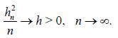
In this Section we will consider the case where the random sample size N_n has the symmetric distribution of the form

where the sequence of natural numbers h_n < n satisfies the condition

that is, h_n = o(n) as n → ∞. It is easy to see that (2.12) and (2.13 imply that N_n / n → 1 in probability as n → ∞.

Lemma 2.2. Let the r.v. Nn have distribution (2.12) under condition (2.13) . Then EN_n = n and, as n → ∞,

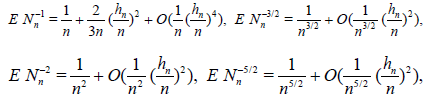
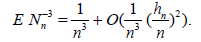
The proof follows from the easily verified equalities

The asymptotic formulas for and are established in a similar way.

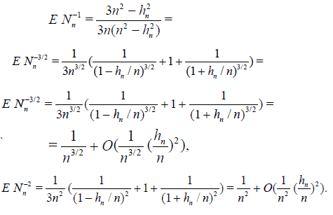
This Lemma and formulas (2.3), (2.6) and (2.9) directly imply the following statement.

Theorem 2.3. Let the r.v. N_n have distribution (2.12) under condition (2.13) . Then,

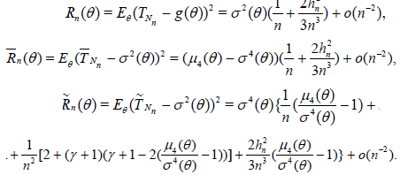
Corollary 2.3. Let the conditions of Theorem 2.3 hold and

Then the asymptotic deficiency of the estimators , and with respect to the corresponding estimators T_n, and has the form

It is worth noting that in Corollary 2.3 h can be arbitrarily large. Therefore the finite asymptotic deficiency d considered in Corollary 2.3 can be arbitrarily large. This is in full correspondence with the conclusion of Section 2.1.

Asymptotic Deficiency and Quantiles

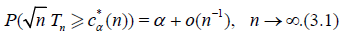
For n ≥ 1 let T_n = T_n(X₁,…, X_n) be a statistic, that is, a measurable function of the r.v.’s X₁,…, X_n. The asymptotic quantile of order α, α ϵ (0, 1) (the α – quantile) of statistic T_n is the value c^*_α (n) for which

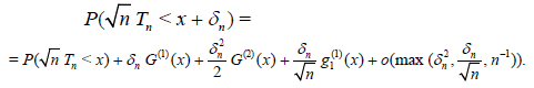
Using Taylor’s formula one has

Lemma 3.1. Suppose that the distribution function of satisfies (uniformly in ) the relation

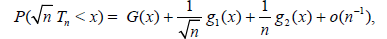
Where, G(x), g₁(x), g₂(x) are sufficiently smooth functions. Then,

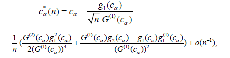
Where, G(c_α) = 1 - α.

Corollary 3.1. Let δn → 0, n → ∞. Then under the conditions of Lemma 3.1 uniformly in

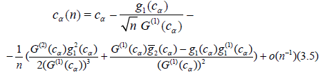
Now consider a statistic S_n = S_n(X₁,…, X_n) other than T_n having α – quantile c_α(n)

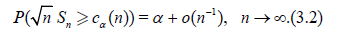
Suppose that:

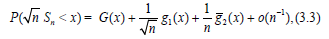
Where, are some smooth functions. Define the sequence of positive integers by the relation ( d is the asymptotic deficiency)

Theorem 3.1. Under the conditions of Lemma 3.1 and (3.3) the asymptotic deficiency d equals

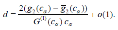
Proof. It follows from (3.1) and Lemma 3.1 that

and

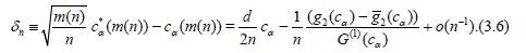
Moreover (3.4) implies

Using Corollary 3.1 we obtain

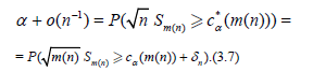
Then (3.2) and (3.6) imply

Now we apply these results to our exapmle.

Let X₁, X₂,… be i.i.d.r.v.’s with

Define

Suppose that the distribution of X₁ satisfies the Cramer condition (C)

Under the conditions (3.8) and (3.10) (see Theorem 6.3.2) we have [8]

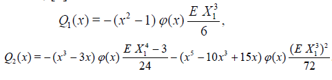
where the functions are defined in [8]

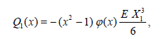
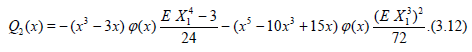
Carrying out the type of computation outlined above we arrive at the following simplified version of Lemma 1.1 (see (3.11)).

Lemma 3.2. Let the conditions (3.8) – (3.10) with k = 3 be satisfied and c^*_α (n) be defined by (3.9), then

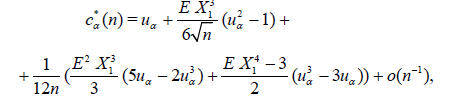
where u_α = Ф^-1(1 – α) denotes the upper α – point of the standard normal distribution.

Now let Y₁, Y₂,… be i.i.d.r.v.’s and

Define

Suppose that

And

Applying Theorem 3.1 we obtain

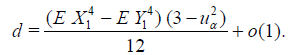
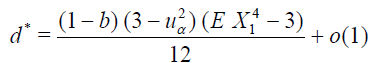
Lemma 3.3. Under the above conditions of Lemma 3.2 and (3.13) - (3.16) the asymptotic deficiency d (see (3.4)) equals

Samples with Random Sizes

Consider random variables N₁, N₂,… è X₁, X₂,…, defined on the same probability space (Ω, A, P). The r.v.’s X₁, X₂,…, X_n will be treated as observations with n being a non-random sample size, whereas the r.v.’s Nn will be treated as random sample size depending on the parameter . For example, if the r.v. N_n has the geometric distribution

then

that is, the r.v. N_n is parametrized by its expectation n.

Assume that for each n ≥ 1 the r.v. N_n takes only natural values, that is, and are independent of the sequence X₁, X₂,…, Everywhere in what follows consider the r.v.’s X₁, X₂,… to be independent and identically distributed. By Hn = Hn(X₁,.., X_n) denote a statistic, that is, real measurable function of observations X₁,.., X_n. For each n ≥ 1 define tne statistic constructed from the sample of random size, that is

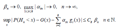
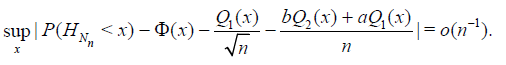
Now assume that the d.f. of the non-normalized statistic H_n admits an asymptotic expansion described by the following condition.

Condition A. There exist constants , , a differentiable d.f. G(x) and measurable functions g_j(x), j = 1,…,k such that

Lemma 4.1. If the condition A holds, then

.

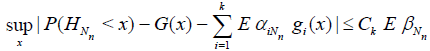The proof is a simple exercise on the application of the formula of total probability.

Let X₁, X₂,… be i.i.d.r.v.’s and

Define for each

. (4.3)

Suppose that the distribution of X₁ satisfies the Cramer condition (C)

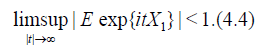
Taking into accopnt (4.2), (4.4) and Theorem 6.3.2 [8] we obtain

, (4.5)

Where, [8]

. (4.6)

Using (4.5) and Lemma 4.1, one has

Lemma 4.2. Let the conditions (4.2) - (4.4) be satisfied, then

.

After these preliminaries (see (4.5) and Lemma 4.2), the following Lemma can be formulated.

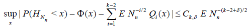
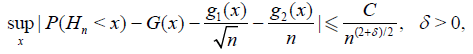
Lemma 4.3. Suppose that the conditions (4.2) - (4.4) hold with k = 4, δ > 0 and there exist a, b such that

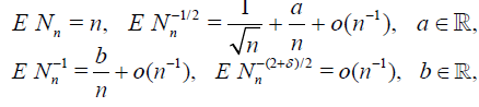
Then,

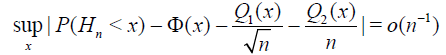
and

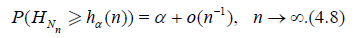
For n ≥ 1 let H_n = H_n (X₁,.., X_n) be a statistic, that is, a measurable function of the r.v.’s X₁,.., X_n. The asymptotic quantile of order α, α ϵ (0, 1) (the α – quantile) of statistic H_n is the value h_α^* (n) for which

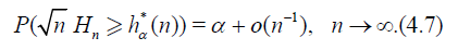
and we consider α – quantile of statistic . That is the value h_α(n) for which

Taking into account (4.5), (4.6) and Lemma 3.1 we obtain

Lemma 4.4. Suppose that the conditions (4.2) - (4.4) hold with k = 4, δ > 0, then under the conditions of Lemma 4.3 α – quantiles h_α^* (n) and h_α(n) admit the following asymptotic expansions

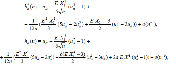
where Ф(u_α) = 1 - α.

Define the sequence of positive integers by the relation (d is the asymptotic deficiency)

Now we have in analogy to Theorem 3.1

Theorem 4.5. Suppose that

and

then the asymptotic deficiency d* (see. (4.9)) satisfies

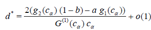
where G(c_α) = 1 - α.

The result of these steps is the following Lemma.

Lemma 4.6. If the conditions of Lemma 4.3 are satisfied, we have (see. (3.12))

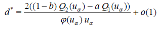
If

.

Then,

Discussion

The case of the samples with random size having a three-point symmetric distribution

In the previous section the results of section 3 were used to solve the main problem of this section. Here we briefly discuss another application of these results (see Lemma 4.2 and Theorem 4.5). Let N_n have a three-point distribution with parameter h_n

(5.1)

where h_n < n and

Lemma 5.1. Let {h_n} be a sequence of positive real numbers with h_n < n and assume that (5.1) and (5.2) hold. Then,

Proof: Here we only sketch the proof. We have:

The proof for the other cases are similar and left to the reader.

Carrying out the type of computation outlined above we arrive at the following simplified version of Lemma 4.1.

Lemma 5.2. Suppose that (4.2) - (4.4) (k = 4 and 0 < δ ≤ 1), (5.1) and (5.2) are satisfied. Then

Corollary 5.2. Under the conditions of Lemma 5.2 we have for h_n = n^3/4 (uniformly in )

The result of these Lemmas is the following Theorem.

Theorem 5.3. If the conditions of Corollary 5.2 are satisfied, we have (see (4.7), (4.8) and (4.9))

where Ф(u_α) = 1 - α and

Conclusion

In the paper we consider asymptotic deficiencies of some estimators based on the samples with random sizes. It can be illustrative characteristic of a possible loss of the accuracy of statistical inference if a random-size-sample is erroneously regarded as a sample with non-random size. Some basic results dealing with some properties of estimators based on the samples with random sizes are also presented.

Acknowledgement

The research is supported by the Russian Foundation for Basic Research, Project 18-07-00252.

2010 Mathematical Subject Classification: Primary 60F05, Secondary 62E20, 91B30, 91B70

References

1. Palfai TP, Monti PM, Ostafin B, Hutchison K (2000) Effects of nicotine deprivation on alcohol-related information processing and drinking behavior. J Abnorm Psychol 109: 96-105.
2. Harrison EL, Hinson RE, McKee SA (2009) Experimenting and daily smokers: episodic patterns of alcohol and cigarette use. Addict Behav 34: 484-486.
3. Howell A, Leyro T, Hogan J, Buckner J, Zvolensky M (2010) Anxiety sensitivity, distress tolerance, and discomfort intolerance in relation to coping and conformity motives for alcohol use and alcohol use problems among young adult drinkers. Addictive Behaviors 35:1144-1147.
4. Krukowski RA, Solomon LJ, Naud S (2005) Triggers of heavier and lighter cigarette smoking in college students. J Behav Med 28: 335-345.
5. Reed MB, Wang R, Shillington AM, Clapp JD, Lange JE (2007) The relationship between alcohol use and cigarette smoking in a sample of undergraduate college students. Addictive Behaviors 32: 449-464.
6. Hughes JR, Kalman D (2006) Do smokers with alcohol problems has more difficulty quitting? Drug Alcohol Depend 82: 91-102.
7. Hurt RD, Offord KP, Croghan IT, Gomez-Dahl L, Kottke TE, et al. (1996) Mortality following inpatient addictions treatment: Role of tobacco use in a community-based cohort. JAMA: Journal of the American Medical Association 275: 1097-1103.
8. Lisha NE, Carmody TP2, Humfleet GL2, Delucchi KL2 (2014) Reciprocal effects of alcohol and nicotine in smoking cessation treatment studies.  Addict Behav 39: 637-643.
9. Taylor B, Rehm J (2006) When risk factors combine: The interaction between alcohol and smoking for aerodigestive cancer, coronary heart disease, and traffic and fire injury. Addictive Behaviors 31: 1522-1535.
10. Jarvis CM, Hayman LL, Braun LT, Schwertz DW, Ferrans CE, et al. (2007) Cardiovascular risk factors and metabolic syndrome in alcohol- and nicotine-dependent men and women. J CardiovascNurs 22: 429-435.
11. Joseph AM, Willenbring ML, Nugent SM, Nelson DB (2004) A randomized trial of concurrent versus delayed smoking intervention for patients in alcohol dependence treatment. Journal of Studies on Alcohol, 65: 681-691.
12. Kodl M, Fu SS, Joseph AM (2006) Tobacco cessation treatment for alcohol-dependent smokers: when is the best time? Alcohol Res Health 29: 203-207.
13. Fu S, Kodl M, Willenbring M, Nelson D, Nugent S, et al. (2008) Ethnic differences in alcohol treatment outcomes and the effect of concurrent smoking cessation treatment. Drug and Alcohol Dependence 92: 61-68.
14. Holt LJ, Litt MD, Cooney NL (2012) Prospective analysis of early lapse to drinking and smoking among individuals in concurrent alcohol and tobacco treatment. Psychology of Addictive Behaviors 26:561-572.
15. Centers for Disease Control and Prevention (CDC) (2009) Cigarette smoking among adults and trends in smoking cessation - United States, 2008. MMWR Morb Mortal Wkly Rep 58: 1227-1232.
16. Irving LM, Seidner AL, Burling TA, Thomas RG, Brenner GF (1994) Drug and alcohol abuse inpatients' attitudes about smoking cessation. J Subst Abuse 6: 267-278.
17. Macnee CL, Talsma A (1995) Development and testing of the barriers to cessation scale. Nurs Res 44: 214-219.
18. Orleans CT, Rimer BK, Cristinzio S, Keintz MK, Fleisher L (1991) A national survey of older smokers: treatment needs of a growing population. Health Psychol 10: 343-351.
19. Kristeller JL (1994) Treatment of hard-core, high-risk smokers using FDA approved pharmaceutical agents: An oral health team perspective. Health Values 18: 25-32.
20. Asher MK, Martin RA, Rohsenow DJ, MacKinnon S, Traficante R, et al. (2003) Perceived barriers to quitting smoking among alcohol dependent patients in treatment. Journal of Substance Abuse Treatment 24: 169-174.
21. Martin RA, Rohsenow DJ, MacKinnon SV, Abrams DB, Monti PM (2006) Correlates of motivation to quit smoking among alcohol dependent patients in residential treatment. Drug Alcohol Depend 83: 73-78.
22. Marlatt GA, Gordon JR (1985) Relapse prevention. New York: Guilford Press.
23. Velicer WF, DiClemente CC, Prochaska JO, Brandenburg N (1985) Decisional balance measure for assessing and predicting smoking status. J PersSoc Psychol 48: 1279-1289.
24. DiClemente CC, Prochaska JO (1982) Self-change and therapy change of smoking behavior: a comparison of processes of change in cessation and maintenance. Addict Behav 7: 133-142.
25. Curry SJ, Grothaus L, McBride C (1997) Reasons for quitting: intrinsic and extrinsic motivation for smoking cessation in a population-based sample of smokers. Addict Behav 22: 727-739.
26. Baha M, Le Faou AL (2010) Smokers' reasons for quitting in an anti-smoking social context. Public Health 124: 225-231.
27. Curry SJ, McBride C, Grothaus LC, Louie D, Wagner EH (1995) A randomized trial of self-help materials, personalized feedback, and telephone counseling with nonvolunteer smokers. J Consult Clin Psychol 63: 1005-1014.
28. Saunders JB, Aasland OG, Babor TF, de la Fuente JR, Grant M (1993) Development of the Alcohol Use Disorders Identification Test (AUDIT): WHO Collaborative Project on Early Detection of Persons with Harmful Alcohol Consumption--II. Addiction 88: 791-804.
29. First MB, Williams JB, Spitzer RL, Gibbon M (2002) Structured Clinical Interview for DSM-IV-TR Axis I Disorders, Clinical Trials Version (SCID-CT). New York: Biometrics Research, New York State Psychiatric Institute.
30. Brown RA, Lejuez CW, Kahler CW, Strong DR (2002) Distress tolerance and duration of past smoking cessation attempts. J Abnorm Psychol 111: 180-185.
31. Heatherton TF, Kozlowski LT, Frecker RC, Fagerström KO (1991) The Fagerström Test for Nicotine Dependence: a revision of the Fagerström Tolerance Questionnaire. Br J Addict 86: 1119-1127.
32. Pomerleau CS, Carton SM, Lutzke ML, Flessland KA, Pomerleau OF (1994) Reliability of the Fagerstrom Tolerance Questionnaire and the Fagerstrom Test for Nicotine Dependence. Addict Behav 19: 33-39.
33. Fagerstrom KO, Heatherton TF, Kozlowski LT (1990) Nicotine addiction and its assessment. Ear Nose Throat J 69: 763-765.
34. Filbey FM, Claus E, Audette AR, Niculescu M, Banich MT, et al. (2007) Exposure to the taste of alcohol elicits activation of the mesocorticolimbicneurocircuitry. Neuropsychopharmacology 33: 1391-1401.
35. Fleming MF, Barry KL, MacDonald R (1991) The alcohol use disorders identification test (AUDIT) in a college sample. Int J Addict 26: 1173-1185.
36. Cherpitel CJ (1995) Analysis of cut points for screening instruments for alcohol problems in the emergency room. J Stud Alcohol 56: 695-700.
37. Macnee CL, Talsma A (1995) Predictors of progress in smoking cessation. Public Health Nurs 12: 242-248.
38. Curry S, Wagner EH, Grothaus LC (1990) Intrinsic and extrinsic motivation for smoking cessation. J Consult Clin Psychol 58: 310-316.
39. McBride CM, Pollak KI, Bepler G, Lyna P, Lipkus IM, et al. (2001) Reasons for quitting smoking among low-income African American smokers. Health Psychol 20: 334-340.
40. Bonn-Miller MO, Zvolensky MJ (2009) An evaluation of the nature of marijuana use and its motives among young adult active users. Am J Addict 18: 409-416.
41. Buckner JD, Zvolensky MJ, Schmidt NB (2012) Cannabis-related impairment and social anxiety: the roles of gender and cannabis use motives. Addict Behav 37: 1294-1297.
42. Agrawal A, Budney AJ, Lynskey MT (2012) The co-occurring use and misuse of cannabis and tobacco: a review. Addiction 107: 1221-1233.
43. Degenhardt L, Hall W, Lynskey M (2001) The relationship between cannabis use and other substance use in the general population. Drug Alcohol Depend 64: 319-327.
44. Cohen J, Cohen P (1983) Applied multiple regression/correlation analysis for the behavioral sciences. Hillsdale, NJ: Lawrence Erlbaum.
45. Cohen J, Cohen P, West SG, Aiken LS (2003) Applied multiple regression/correlation analysis for the behavioral sciences (3rd ed.). Mahwah, NJ US: Lawrence Erlbaum Associates Publishers.
46. Lipkus IM, Feaganes JR, Green JD, Sedikides C (2001) The Relationship Between Attitudinal Ambivalence and Desire to Quit Smoking Among College Smokers. Journal of Applied Social Psychology, 31: 113-133.
47. Wilson SJ, Creswell KG, Sayette MA, Fiez JA (2013) Ambivalence about smoking and cue-elicited neural activity in quitting-motivated smokers faced with an opportunity to smoke.  Addict Behav 38: 1541-1549.
48. Festinger LA (1957) A theory of cognitive dissonance. Evanston, IL: Row, Peterson.
49. Markowitz LJ (2000) Smoker's perceived self-exemption from health risks. Psi Chi Journal of Undergraduate Research 5: 119-124.
50. Jamieson P, Romer D (2001)What do young people think they know about the risks of smoking? In P. Slovic (Ed.), Smoking: Risk, perception, and policy (pp. 51-63). Thousand Oaks, CA US: Sage Publications, Inc.
51. Schane RE, Glantz SA, Ling PM (2009) Social smoking implications for public health, clinical practice, and intervention research. American Journal of Preventive Medicine 37: 124-131.
52. DaniJA, De Biasi M (2001) Cellular mechanisms of nicotine addiction. PharmacolBiochemBehav 70: 439-446.
53. Nestler EJ (2005) Is there a common molecular pathway for addiction? Nat Neurosci 8: 1445-1449.
54. Ehrman RN, Robbins SJ, Bromwell MA, Lankford ME, Monterosso JR, et al. (2002) Comparing attentional bias to smoking cues in current smokers, former smokers, and non-smokers using a dot-probe task. Drug Alcohol Depend 67: 185-191.
55. Kerst WF, Waters AJ (2014)Attentional retraining administered in the field reduces smokers’ attentional bias and craving.
56. Wiers RW, Rinck M, Kordts R, Houben K, Strack F (2010) Retraining automatic action-tendencies to approach alcohol in hazardous drinkers. Addiction 105: 279-287.
57. Raupach T, West R, Brown J (2013) The most "successful" method for failing to quit smoking is unassisted cessation. Nicotine Tob Res 15: 748-749.
58. Korte KJ, Capron DW, Zvolensky M, Schmidt NB (2013) The Fagerström test for nicotine dependence: do revisions in the item scoring enhance the psychometric properties? Addict Behav 38: 1757-1763.