Research Article - Biomedical Research (2017) Health Science and Bio Convergence Technology: Edition-II
Design and development of an efficient hierarchical approach for multi-label protein function prediction
Mohana Prabha G1* and Chitra S2
1M. Kumarasamy College of Engineering, Karur, Tamil Nadu, India
2Er. Perumal Manimekalai College of Engineering, Hosur, Tamil Nadu, India
Accepted on November 14, 2016
Abstract
Protein function prediction is important for understanding life at the molecular level and therefore is highly demanded by biomedical research and pharmaceutical applications. To overcome the problem, in this work I have proposed a novel multi-label protein function prediction based on hierarchical approach. In Hierarchical multi-label classification problems, each instance can be classified into two or more classes simultaneously, differently from conventional classification. Mainly, the proposed methodology is consisting of three phases such as (i) Creating clusters (ii) Generation of class vectors and (iii) classification of instances. At first, we create the clusters based on the hybridization of KNearest Neighbor and Expectation Maximization algorithm (KNN+EM). Based on the clusters we generate the class vectors. Finally, protein function prediction is carried out in the classification stage. The performance of the proposed method is extensively tested upon five types of protein datasets, and it is compared to those of the two methods in terms of accuracy. Experimental results show that our proposed multi-label protein function prediction significantly superior to the existing methods over different datasets.
Keywords
Protein function prediction, Bio-medical, Multi-label, KNN+EM, Hierarchical
Introduction
Mining data streams is a real time process of extracting interesting patterns from high-speed data streams. Clustering is an important class in data stream mining in which analogous objects are categorized in one cluster. Traditional clustering algorithms are not applicable in data streams. Several clustering algorithms are developed recently for clustering data streams [1-4]. Some of these clustering algorithms apply a distance function for determining similarity between objects in a cluster. Another group of the clustering methods are grid-based clustering. The grid-based clustering method uses a multi resolution grid data structure. It forms the grid data structure by dividing the data space into a number of cells and perform the clustering on the grids [5]. Classification is an important theme in data mining. Classification is a process to assign a class to previously unseen data as accurately as possible. The unseen data are those records whose class value is not present and using classification, class value is predicted. In order to predict the class value, training set is used. Training set consists of records and each record contains a set of attributes, where one of the attribute is the class. From training set a classifier is created. Then that classifier’s accuracy is determined using test set. If accuracy is acceptable then and only then classifier is used to predict class value of unseen data. Label-based methods, such as label ranking and label classification, play important roles in clustering. Classification can be divided in two types: single-label classification and multi-label classification.
Single-label classification is to learn from a set of instances, each associated with a unique class label from a set of disjoint class labels L. Multi-label classification is to learn from a set of instances where each instance belong to one or more classes in L. Text data sets can be binary, multi-class or multi-label in nature. For the first two categories, only a single class label can be associated with a document. However, in case of multi label data, more than one class labels can be associated with a document at the same time. However, even if a data set is multi-label, not all combinations of class-labels appear in a data set. Also, the probability with which a particular class label combination occurs is also different. It indicates that there is a correlation among the different class-labels and it varies across each pair of class labels. If we look into the literature for multi-label classification, we can see that most traditional approaches try to transform the multi-label problem to multi-class or binary class problem. For example, if there is T class labels in the multi-label problem, one binary SVM (i.e., one vs. rest SVM) classifier can be trained for each of the class labels and the classification results of these classifiers can be merged to get the final prediction. But, this does not provide a correct interpretation of the data [6]. Because, if a data point belongs to more than one class, then during binary SVM training, it may belong to both the positive and negative classes at the same time.
Multi-label classification is a variant of the classification problem in which multiple target labels must be assigned to each instance. This method has been widely employed in recent years [7] and describing samples with labels is a challenging task [8]. A number of computational protein function prediction methods had been developed in the last few decades [9-12]. The most commonly used method is to use the tool Basic Local Alignment Search Tool (BLAST) [13] to search a query sequence against protein databases containing experimentally determined function annotations to retrieve the hits based on the sequence homology. The huge amount of biological data has to be stored, analysed, and retrieved. Protein databases are categorized as primary or structural [14]. Primary protein databases contain protein sequences. Example of these databases is SWISS-PROT [15]. SWISS-PROT annotates the sequences as well as describing the protein functions. Structural databases contain molecular structures. The Protein Data Bank PDB [16] is the main database for three dimensional structures of molecules specified by X-ray crystallography and NMR (nuclear magnetic resonance). Moreover, Proteins functions are related to their structural role or enzymatic role [17]. The structural role is related to forming the cell shape. The enzymatic role is related to help in accomplishing chemical reactions, signal movement in and out of the cell and transportation of different kind of molecules like antibodies, structural binding elements, and movement-related motor elements.
In this paper, we propose a multi-label protein function prediction based on hybridization of k-Nearest Neighbor based EM algorithm (KNN+EM). The main idea is to reduce the number of data with KNN method and guess the class using most similar training data with EM algorithm. Based on the algorithm multi-label protein function prediction is carried out. The rest of the paper is organized as follows: In section 2 we present the some of the related work present in the protein function prediction and in section 3 we deeply describe the proposed protein function prediction method. The section 4, we explained the experimental results and performance evaluation and in section 5 we discuss the conclusion part.
Related Works
Many of the researchers have explained the bio-information based protein function prediction. Among them some of the research papers explained in this section; Fahimeh et al. [18] have explained the variance reduction based binary fuzzy decision tree induction method for protein function prediction. Protein Function Prediction (PFP) was one of the special and complex problems in machine learning domain in which a protein (regarded as instance) may have more than one function simultaneously. This algorithm just fuzzifies the decision boundaries instead of converting the numeric attributes into fuzzy linguistic terms. It has the ability of assigning multiple functions to each protein simultaneously and preserves the hierarchy consistency between functional classes. It uses the label variance reduction as splitting criterion to select the best “attribute-value” at each node of the decision tree. The experimental results were show that the overall performance of the algorithm was promising.
Moreover, Wei et al. have explained the active learning for protein function prediction in protein-protein interaction networks [19]. The high-throughput technologies have led to vast amounts of Protein-Protein Interaction (PPI) data, and a number of approaches based on PPI networks were explained for protein function prediction. However, these approaches do not work well if annotated or labelled proteins are scarce in the networks. To address this issue, they explained this method. They, first cluster a PPI network by using the spectral clustering algorithm and select some informative candidates for labelling within each cluster according to a certain centrality metric, and then apply a collective classification algorithm to predict protein function based on these labelled proteins. Experiments over two real datasets demonstrate that the active learning based approach achieves a better prediction performance by choosing more informative proteins for labelling.
Additionally, Ernando et al. have explained the hierarchical multi-label classification ant colony algorithm for protein function prediction [20]. This paper explained the hierarchical multi-label classification problem of protein function prediction. This problem was a very active research field, given the large increase in the number of un-characterized proteins available for analysis and the importance of determining their functions in order to improve the current biological knowledge. In this type of problem, each example may belong to multiple class labels and class labels are organized in a hierarchical structure either a tree or a Directed Acyclic Graph (DAG) structure. It presents a more complex problem than conventional flat classification, given that the classification algorithm has to take into account hierarchical relationships between class labels and be able to predict multiple class labels for the same example. Their ACO algorithm discovers an ordered list of hierarchical multi-label classification rules. It was evaluated on sixteen challenging bioinformatics data sets involving hundreds or thousands of class labels to be predicted and compared against state-of-theart decision tree induction algorithms for hierarchical multilabel classification.
Similarly, Guoxian et al. have explained the protein function prediction using multilabel ensemble classification [21]. High-throughput experimental techniques produce several kinds of heterogeneous proteomic and genomic data sets. To computationally annotate proteins, it is necessary and promising to integrate these heterogeneous data sources. In this paper they developed a Transductive Multilabel Classifier (TMC) to predict multiple functions of proteins using several unlabelled proteins. They also explained a method called Transductive Multilabel Ensemble Classifier (TMEC) for integrating the different data sources using an ensemble approach. The TMEC trains a graph-based multilabel classifier on each single data source, and then combines the predictions of the individual classifiers. They used a directed birelational graph to capture the relationships between pairs of proteins, between pairs of functions, and between proteins and functions. They, evaluate the effectiveness of the TMC and TMEC to predict the functions of proteins on three benchmarks.
Guoxian et al. have explained the Predicting Protein Function Using Multiple Kernels (ProMK) [22]. ProMK iteratively optimizes the phases of learning optimal weights and reduces the empirical loss of multi-label classifier for each of the labels simultaneously. ProMK was integrating kernels selectively and downgrade the weights on noisy kernels. They investigate the performance of ProMK on several publicly available protein function prediction benchmarks and synthetic datasets. They show that their approach performs better than previously proposed protein function prediction approaches that integrate multiple data sources and multi-label multiple kernel learning methods.
Moreover, Xiao et al. have explained the framework for incorporating functional interrelationships into protein function prediction algorithms [23]. In this study, they explained a functional similarity measure in the form of Jaccard coefficient to quantify these interrelationships and also develop a framework for incorporating GO term similarity into protein function prediction process. The experimental results of crossvalidation on S. Cerevisiae and Homo sapiens data sets demonstrate that their method was able to improve the performance of protein function prediction. In addition, they find that small size terms associated with a few of proteins obtain more benefit than the large size ones when considering functional interrelationships. They also compare their similarity measure with other two widely used measures, and results indicate that when incorporated into function prediction algorithms, their measure was more effective.
Proposed Multi Label Protein Function Prediction
The main objective of this paper is to multi label protein function prediction based on hybridization of k-Nearest Neighbor and EM algorithm (KNN+EM). The multi label classification is carried out by training, validation and testing sequences. The multi label classification requires a set of Z-dimensional training instances as input and it is denoted as and test instances as of class labels represented as in which in a k-class problem for the instance. At first, the training instances are taken and create clusters based on the (KNN+EM) algorithm and these instances are placed in an appropriate cluster by calculating the most probable cluster. The validation or unseen instances are classified based on the threshold by generating a class vector for each cluster. At last, the testing instances are classified as the final prediction. The multi label classification is carried out by the three steps such as (i) creating clusters based on (KNN+EM), (ii) Generation of class vectors and (iii) classification of instances and is explained below in detail. The overall diagram of proposed methodology is illustrated in Figure 1.

Figure 1. Overall diagram of the proposed methodology.
Creating clusters based on HKNNEM
The first step is to create clusters for the training dataset (R) which is comprised of (z) attributes and (Z) instances. By using the HKNNEM algorithm, it helps to reduce the number of data with KNN method and guess the class using most similar training data with EM algorithm. The proposed HKNNEM algorithm is explained as follows:
A. HKNNEM algorithm: The HKNNEM algorithm is a hybrid approach which is the combination of KNN and EM algorithm. In K-Nearest Neighbor (KNN), the data set is clustered many times using a KNN clustering with a simple strategy. The goal is to combine similar classes that are close to each other. KNN clustering algorithm searches the training samples that are nearest to the new sample as the new sample neighbours, which cluster includes most of these k samples, then predict the cluster label of x is same with this cluster. In Expectation Maximization (EM) algorithm, is one of the Bayesian methods which are based on probability calculus. EM is to form Gaussian distributions for each class and predict the class of queried data. EM algorithm is a method to guess units which has missing data and includes maximum similarity probabilities. EM method is a repeated method with two stages. Expectation stage gives expectation for the data. Maximization stage gives expectation about mean, standard deviation or correlation when a missing data is appointed. This process continues until the change on expected values decreases to a negligible value. The EM algorithm is a general approach to maximum likelihood in the presence of incomplete data. It is utilized for unknown values with known probability distributions. The hybrid approach of KNN and EM is proposed in this paper. The steps involved in the process of HKNNEM algorithm is as follows:
Step 1: At first, we read the training and testing data from a file. These data are used one by one for training and testing purposes. Training mode is interactive and no batch mode exists. Let R={r1, r2, r3….rz} be the train data set where each ri belongs to i=1-z is a vector and V is the test vector.
Step 2: After that, the number of class in the data set is identified and the data of the data set is divided into groups according to their classes, because the data set consists of list of classes and each class is denoted by a class number.
Step 3: Then distances between training and testing data are calculated by using selected distance measurement. Let where D={d1, d2, d3….dz} is the distance matrix. Each di is denoted by i=1-z and which is the difference between each train and test data. Different distance measurements can be used for distance calculations. In this paper, the distance is calculated by using the following equation.
 (1)
(1)
Where; is the Minkowski distance. Here, when is equal to 1, it is called as Manhattan distance, for is equal to 2, it is called as Euclidean distance. If is equal to 3 or more, the general name Minkowski is used for that distance. The value of is chosen in the order of 1, 2 and 3. From these the best value for is chosen and based on that the distance formula is decided.
Step 4: After that, for each class group, the calculated distances are sorted in ascending order. In this case, we obtain the minimum distance means; it indicates more similar data’s are present in the testing data. The formula for applying the sorting process is as follows.
 (2)
(2)
Step 5: In this step, we have to choose the optimum k data that have minimum distance to the test data from each class to form a new test data. This is determined heuristically considering the distances between queried and train data for the KNN algorithm. Thus the k-nearest neighbours is found for the training data set. After that point old train set is updated with the new one as shown in equation.
 (3)
(3)
Where; h=1-k. Thus the training instances which are close to one other are obtained. Now for these training instances the EM algorithm is applied.
Step 6: For the initialization process, assume that it consists of M classes and each class is represented as is constituted by a parameter vector (v), composed by the mean (μe) and by the covariance matrix (Cε), which represents the features of the Gaussian probability distribution (Normal) used to characterize the observed and unobserved entities of the data set R.
 (4)
(4)
On the initial instant (t=0) the implementation can generate randomly the initial values of mean (μe) and of covariance matrix (Cε). The EM algorithm aims to approximate the parameter vector (v) of the real distribution. Another alternative offered by MCLUST is to initialize EM with the clusters obtained by a hierarchical clustering technique.
Step 7: In this expectation step, it is responsible to estimate the probability of each element belong to each cluster (P (Gε ׀ ri)) by assuming the parameters of each of the k distributions are already known. The relevance degree of the points of each cluster is given by the likelihood of each element attribute in comparison with the attributes of the other elements of cluster Gε.
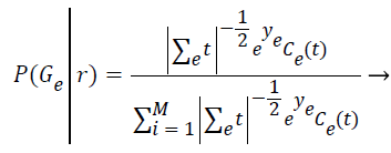 (5)
(5)
Step 8: The Maximization step is responsible to estimate the parameters of the probability distribution of each class for the next step. First is computed the mean (μe) of class e obtained through the mean of all points in function of the relevance degree of each point.
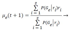 (6)
(6)
Step 9: To find the covariance matrix for the next iteration is applied the Bayes Theorem based on the conditional probabilities of the class occurrence. This implies that P (A ׀ B)=P (B ׀ A)*P (A) P (B). Thus the covariance is computed as follows:
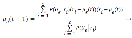 (7)
(7)
Step 10: The probability of occurrence of each class is computed through the mean of probabilities (Gε) in function of the relevance degree of each point from the class.
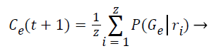 (8)
(8)
The attributes represents the parameter vector (v) that characterize the probability distribution of each class that will be used in the next algorithm iteration.
Step 11: The iteration between the expectation and maximization steps is performed until one of the two conditions occurs:
• The maximum number of 100 iterations is reached; or
• The difference between the log-likelihood of two consecutive steps is smaller than 1 × 10⁻⁶
The log-likelihood is computed after each expectation step:
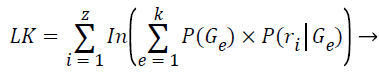 (9)
(9)
Step 12: After performing all the iteration it is necessary to perform the convergence test. It verifies if the difference of the attributes vector of iteration to the previous iteration is smaller than an acceptable error tolerance, given by parameter. Some implementations use the difference between the averages of class distribution as the convergence criterion.
Step 13: After the algorithm has converged and the final parameters of the k clusters are known, the Z training instances are assigned to their most probable cluster.
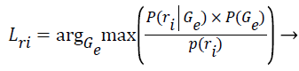 (10)
(10)
Generation of class vector
Once the training instances have been distributed throughout the clusters, we generate one class vector per cluster. By using the two strategies, we generate one class vector per cluster based on the literature Barros et al. [24]. We follow the paper for generating the class vector based on the threshold.
1). The class vector of cluster Gε is generated as the average class vector of the training instances that were assigned to cluster Gε, i.e.:
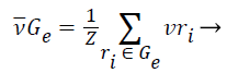 (11)
(11)
2). The class vector of cluster is generated as the average class vector of the training instances that were assigned to cluster and whose cluster membership probability surpasses a given previously-defined threshold Δe, i.e.:
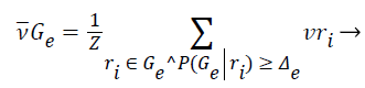 (12)
(12)
Note that strategy 1 is a special case of strategy 2 in which Δ=0 for all clusters. The second strategy, on the other hand, makes use of the cluster memberships to define the average class vectors. We also distribute the validation instances to their most probable cluster, also according to Equation 10. Then, for each cluster, we evaluate the classification performance of the validation instances with the area under the precision-recall curve by building the average class vector following Equation 12. For that, we have to try different values of Δe i.e. {0, 0.1, 0.2, 0.3, 0.4, 0.5, 0.6, 0.7, 0.8, and 0.9}. The average class vector built according to the threshold value that yielded the largest AUPRC value is then chosen to classify the test instances that are assigned to cluster Gε.
Classification of instances
The classification is used to classify the test instances. The classification is done based on the following assumptions.
i. Assign each test instance to its most probable cluster according to Equation 10;
ii. Assuming test instance was assigned to cluster, make use of class vector computed from the training instances that belong to cluster and have cluster membership probability greater than as the class prediction for test instance.
The algorithm for our proposed HKNNEM is explained below.
| Input: |
| Training dataset R, Testing data S |
| Start: |
| Set threshold ts={0, 0.1, 0.2, 0.3, 0.4, 0.5, 0.6, 0.7, 0.8, 0.9} |
| Divide R in to training set Rt and validation set Rv |
| Get all train and test data |
| Calculate distances ‘D’ between each train and test data |
| Sort (D, R) in ascending order for each class |
| For i=1 to n |
| For j=1 to n-1 |
| If Di+1<Di |
| Temp_D= Di |
| Di=Di+1 |
| Di+1=Temp_D |
| Temp_X=Xi |
| Xi=Xi+1 |
| Xi+1=temp_X |
| End if |
| End for |
| End for |
| Choose k data that have minimum distances to the test data from each class to form a new dataset |
| Replace old dataset by new dataset |
| Calculate probability of each cluster based on instance |
| K ← CV (Rt) |
| Partition ← EM ( Rt, k) |
| For ri ε Rt do |
| Lri ← equation 10 |
| end for |
| For ri ε Rv do |
| Lri ← equation 10 |
| end for |
| for cluster Gε ε ts do |
| Best AUPRC ← 0 |
| For △ε ε ts do |
| vGε ← equation 12 |
| AUPRC ← classify ({riv | riv ε Gε} v Gε) |
| If AUPRC ≥ bestAUPRC then |
| thresholdε ← △ε |
| end if |
| end for |
| end for |
| partition ← EM (Rt∪ Rv, k) |
| return thresholds, partition |
| end |
Result and Discussion
In this section, we discuss the result obtained from the proposed multi-label protein function prediction. We have implemented our proposed work using Java (jdk 1.6) with cloud Sim tools and a series of experiments were performed on a PC with Windows 7 Operating system at 2 GHz dual core PC machine with 4 GB main memory running a 64-bit.
Datasets description
Protein function prediction datasets are used in this approach [25]. Here, we used five types of dataset such as cellcycle, derisi, eisen, gasch1 and gasch 2. Cell cycle dataset contains 77 attributes and 4125 classes. The EISEN dataset contains the totally 61 attributes and 4119 classes. The DERISI dataset contains the 79 attributes and 3573 classes. The GASCH 1and GASCH 2 contains 173 and 52 attributes and 4125 and 4131 classes respectively. These datasets are related to issues like phenotype data and gene expression levels. Table 1 summarizes the main characteristics of the training, validation, and test datasets employed in the experiments.
| Structure | Dataset | Attributes | Classes | Training | Validation | Testing | |||
|---|---|---|---|---|---|---|---|---|---|
| Total | Multi | Total | Multi | Total | Multi | ||||
| DAG | Cell cycle | 77 | 4125 | 1625 | 1625 | 848 | 848 | 1278 | 1278 |
| EISEN | 79 | 4119 | 1605 | 1605 | 842 | 842 | 1272 | 1272 | |
| DERISI | 63 | 3573 | 1055 | 1055 | 528 | 528 | 835 | 835 | |
| GASCH1 | 173 | 4125 | 1631 | 1631 | 846 | 846 | 1281 | 1281 | |
| GASCH2 | 52 | 4131 | 1636 | 1636 | 849 | 849 | 1288 | 1288 | |
Table 1. Summary of dataset.
Evaluation metrics
The experiential result is evaluated based on the accuracy, sensitivity and specificity. The experimentation is carried out based on training, validation and testing performance.
Sensitivity: The sensitivity of the multi-label protein function prediction is determined by taking the ratio of number of true positives to the sum of true positive and false negative. This relation can be expressed as.
Specificity: The specificity of the feature multi-label protein function prediction can be evaluated by taking the relation of number of true negatives to the combined true negative and the false positive. The specificity can be expressed as
Accuracy: The accuracy of multi-label protein function prediction can be calculated by taking the ratio of true values present in the population. The accuracy can be described by the following equation
Where, represents the True positive, represents the True negative, represents the false positive and represents the False negative.
Experimental results
The basic idea of proposed methodology is multi-label protein function prediction based on hierarchical approach. This approach is based on combination of EM and K-means clustering algorithm. In this section, we compare our proposed protein function prediction with Hierarchical Multi-Label Classification with Probabilistic Clustering (HMC-PC) and two decision tree-based local methods, namely Clus-HSC [26]. HMC-PC works by clustering the protein function datasets in k clusters following an expectation-maximization scheme. Then, for each of the k clusters, the average class vector is generated based on the training instances that were (hard-) assigned to each cluster. The choice of which instances will be used to define the per-cluster average class vector is based on the probabilities of cluster membership. The proposed methodology is compare to the HMC-PC method. Tables 2-4 show the performance comparison of proposed methodology based on accuracy, specificity and sensitivity.
| Dataset | Class | Proposed | HMC-PC | Clus-HSC | Class | Proposed | HMC-PC | Clus-HSC |
|---|---|---|---|---|---|---|---|---|
| Cell cycle | GO: 0044464 | 0.959 | 0.921 | 0.917 | GO: 0044424 | 0.928 | 0.921 | 0.898 |
| GO: 0009987 | 0.88 | 0.876 | 0.86 | GO: 0008152 | 0.78 | 0.767 | 0.726 | |
| GO: 0003735 | 0.71 | 0.649 | 0.404 | GO: 0044237 | 0.701 | 0.699 | 0.676 | |
| GO: 0044238 | 0.702 | 0.677 | 0.65 | GO: 0044444 | 0.635 | 0.624 | 0.586 | |
| GO: 0043170 | 0.663 | 0.632 | 0.58 | GO: 0006412 | 0.62 | 0.599 | 0.361 | |
| EISEN | GO: 0044464 | 0.985 | 0.953 | 0.941 | GO: 0044424 | 0.928 | 0.901 | 0.926 |
| GO: 0009987 | 0.91 | 0.9 | 0.916 | GO: 0008152 | 0.72 | 0.713 | 0.692 | |
| GO: 0003735 | 0.82 | 0.84 | 0.808 | GO: 0044237 | 0.69 | 0.687 | 0.636 | |
| GO: 0044238 | 0.68 | 0.652 | 0.607 | GO: 0044444 | 0.79 | 0.77 | 0.751 | |
| GO: 0043170 | 0.75 | 0.726 | 0.716 | GO: 0006412 | 0.75 | 0.72 | 0.664 | |
| DERISI | GO: 0044464 | 0.968 | 0.934 | 0.965 | GO: 0044424 | 0.89 | 0.88 | 0.888 |
| GO: 0009987 | 0.84 | 0.838 | 0.849 | GO: 0008152 | 0.74 | 0.736 | 0.736 | |
| GO: 0003735 | 0.68 | 0.668 | 0.674 | GO: 0044237 | 0.66 | 0.643 | 0.643 | |
| GO: 0044238 | 0.61 | 0.55 | 0.582 | GO: 0044444 | 0.46 | 0.41 | 0.462 | |
| GO: 0043170 | 0.62 | 0.556 | 0.585 | GO: 0006412 | 0.59 | 0.52 | 0.525 | |
| GASCH1 | GO: 0044464 | 0.96 | 0.958 | 0.963 | GO: 0044424 | 0.92 | 0.927 | 0.912 |
| GO: 0009987 | 0.86 | 0.845 | 0.855 | GO: 0008152 | 0.63 | 0.614 | 0.659 | |
| GO: 0003735 | 0.74 | 0.754 | 0.733 | GO: 0044237 | 0.72 | 0.699 | 0.674 | |
| GO: 0044238 | 0.61 | 0.583 | 0.574 | GO: 0044444 | 0.71 | 0.671 | 0.66 | |
| GO: 0043170 | 0.65 | 0.639 | 0.647 | GO: 0006412 | 0.68 | 0.659 | 0.616 | |
| GASCH2 | GO: 0044464 | 0.96 | 0.951 | 0.966 | GO: 0044424 | 0.92 | 0.926 | 0.91 |
| GO: 0009987 | 0.86 | 0.85 | 0.863 | GO: 0008152 | 0.63 | 0.609 | 0.622 | |
| GO: 0003735 | 0.74 | 0.739 | 0.741 | GO: 0044237 | 0.71 | 0.682 | 0.696 | |
| GO: 0044238 | 0.61 | 0.536 | 0.521 | GO: 0044444 | 0.69 | 0.668 | 0.667 | |
| GO: 0043170 | 0.68 | 0.669 | 0.655 | GO: 0006412 | 0.64 | 0.619 | 0.601 |
Table 2. Performance of protein function prediction based on the accuracy.
| Dataset | Class | Proposed | HMC-PC | Clus-HSC | Class | Proposed | HMC-PC | Clus-HSC |
|---|---|---|---|---|---|---|---|---|
| Cell cycle | GO: 0044464 | 0.84 | 0.8 | 0.71 | GO: 0044424 | 0.84 | 0.82 | 0.8 |
| GO: 0009987 | 0.75 | 0.76 | 0.6 | GO: 0008152 | 0.67 | 0.66 | 0.64 | |
| GO: 0003735 | 0.6 | 0.63 | 0.56 | GO: 0044237 | 0.58 | 0.55 | 0.54 | |
| GO: 0044238 | 0.59 | 0.6 | 0.51 | GO: 0044444 | 0.51 | 0.46 | 0.5 | |
| GO: 0043170 | 0.57 | 0.56 | 0.77 | GO: 0006412 | 0.51 | 0.45 | 0.47 | |
| EISEN | GO: 0044464 | 0.86 | 0.8 | 0.3 | GO: 0044424 | 0.81 | 0.78 | 0.8 |
| GO: 0009987 | 0.79 | 0.79 | 0.6 | GO: 0008152 | 0.62 | 0.6 | 0.61 | |
| GO: 0003735 | 0.75 | 0.73 | 0.5 | GO: 0044237 | 0.59 | 0.58 | 0.6 | |
| GO: 0044238 | 0.56 | 0.55 | 0.56 | GO: 0044444 | 0.68 | 0.65 | 0.64 | |
| GO: 0043170 | 0.65 | 0.64 | 0.77 | GO: 0006412 | 0.63 | 0.62 | 0.61 | |
| DERISI | GO: 0044464 | 0.84 | 0.82 | 0.73 | GO: 0044424 | 0.75 | 0.73 | 0.74 |
| GO: 0009987 | 0.73 | 0.71 | 0.61 | GO: 0008152 | 0.62 | 0.6 | 0.61 | |
| GO: 0003735 | 0.59 | 0.6 | 0.5 | GO: 0044237 | 0.58 | 0.55 | 0.6 | |
| GO: 0044238 | 0.59 | 0.56 | 0.53 | GO: 0044444 | 0.42 | 0.4 | 0.4 | |
| GO: 0043170 | 0.52 | 0.51 | 0.52 | GO: 0006412 | 0.49 | 0.46 | 0.45 | |
| GASCH1 | GO: 0044464 | 0.79 | 0.77 | 0.72 | GO: 0044424 | 0.79 | 0.75 | 0.72 |
| GO: 0009987 | 0.74 | 0.54 | 0.6 | GO: 0008152 | 0.61 | 0.6 | 0.63 | |
| GO: 0003735 | 0.63 | 0.6 | 0.64 | GO: 0044237 | 0.7 | 0.69 | 0.7 | |
| GO: 0044238 | 0.52 | 0.5 | 0.53 | GO: 0044444 | 0.6 | 0.6 | 0.59 | |
| GO: 0043170 | 0.57 | 0.56 | 0.6 | GO: 0006412 | 0.59 | 0.58 | 0.54 | |
| GASCH2 | GO: 0044464 | 0.78 | 0.77 | 0.8 | GO: 0044424 | 0.79 | 0.77 | 0.7 |
| GO: 0009987 | 0.75 | 0.73 | 0.72 | GO: 0008152 | 0.59 | 0.6 | 0.58 | |
| GO: 0003735 | 0.64 | 0.61 | 0.62 | GO: 0044237 | 0.64 | 0.63 | 0.61 | |
| GO: 0044238 | 0.52 | 0.5 | 0.53 | GO: 0044444 | 0.58 | 0.55 | 0.54 | |
| GO: 0043170 | 0.55 | 0.53 | 0.54 | GO: 0006412 | 0.53 | 0.5 | 0.53 |
Table 3. Performance of protein function prediction based on the specificity.
| Dataset | Class | Proposed | HMC-PC | Clus-HSC | Class | Proposed | HMC-PC | Clus-HSC |
|---|---|---|---|---|---|---|---|---|
| Cell cycle | GO: 0044464 | 0.96 | 0.86 | 0.69 | GO: 0044424 | 0.93 | 0.85 | 0.75 |
| GO: 0009987 | 0.89 | 0.83 | 0.65 | GO: 0008152 | 0.79 | 0.7 | 0.6 | |
| GO: 0003735 | 0.73 | 0.71 | 0.66 | GO: 0044237 | 0.74 | 0.71 | 0.61 | |
| GO: 0044238 | 0.72 | 0.72 | 0.62 | GO: 0044444 | 0.71 | 0.68 | 0.62 | |
| GO: 0043170 | 0.68 | 0.65 | 0.64 | GO: 0006412 | 0.7 | 0.65 | 0.68 | |
| EISEN | GO: 0044464 | 0.98 | 0.91 | 0.75 | GO: 0044424 | 0.94 | 0.9 | 0.71 |
| GO: 0009987 | 0.93 | 0.87 | 0.62 | GO: 0008152 | 0.76 | 0.7 | 0.75 | |
| GO: 0003735 | 0.9 | 0.84 | 0.72 | GO: 0044237 | 0.76 | 0.75 | 0.75 | |
| GO: 0044238 | 0.72 | 0.69 | 0.74 | GO: 0044444 | 0.81 | 0.8 | 0.82 | |
| GO: 0043170 | 0.8 | 0.75 | 0.81 | GO: 0006412 | 0.78 | 0.76 | 0.71 | |
| DERISI | GO: 0044464 | 0.98 | 0.92 | 0.73 | GO: 0044424 | 0.92 | 0.85 | 0.76 |
| GO: 0009987 | 0.86 | 0.82 | 0.7 | GO: 0008152 | 0.83 | 0.82 | 0.8 | |
| GO: 0003735 | 0.73 | 0.69 | 0.72 | GO: 0044237 | 0.76 | 0.75 | 0.68 | |
| GO: 0044238 | 0.69 | 0.65 | 0.55 | GO: 0044444 | 0.59 | 0.6 | 0.59 | |
| GO: 0043170 | 0.71 | 0.66 | 0.59 | GO: 0006412 | 0.67 | 0.61 | 0.6 | |
| GASCH1 | GO: 0044464 | 0.98 | 0.92 | 0.87 | GO: 0044424 | 0.95 | 0.92 | 0.89 |
| GO: 0009987 | 0.9 | 0.84 | 0.82 | GO: 0008152 | 0.71 | 0.72 | 0.7 | |
| GO: 0003735 | 0.81 | 0.75 | 0.74 | GO: 0044237 | 0.76 | 0.71 | 0.7 | |
| GO: 0044238 | 0.7 | 0.62 | 0.65 | GO: 0044444 | 0.78 | 0.75 | 0.76 | |
| GO: 0043170 | 0.76 | 0.72 | 0.71 | GO: 0006412 | 0.76 | 0.75 | 0.74 | |
| GASCH2 | GO: 0044464 | 0.97 | 0.91 | 0.89 | GO: 0044424 | 0.93 | 0.87 | 0.86 |
| GO: 0009987 | 0.91 | 0.86 | 0.9 | GO: 0008152 | 0.76 | 0.71 | 0.7 | |
| GO: 0003735 | 0.8 | 0.73 | 0.79 | GO: 0044237 | 0.79 | 0.7 | 0.69 | |
| GO: 0044238 | 0.69 | 0.7 | 0.7 | GO: 0044444 | 0.72 | 0.64 | 0.63 | |
| GO: 0043170 | 0.76 | 0.72 | 0.73 | GO: 0006412 | 0.7 | 0.58 | 0.57 |
Table 4. Performance of protein function prediction based on the sensitivity.
The above Table 2 shows the Performance comparison of protein function prediction based on the accuracy. Here, we used five types of protein function dataset. When using the Cell cycle dataset we obtain the maximum accuracy of 0.959 which is 0.921 for using HMC-PC and 0.917 for using Clus- HMC based protein function prediction. When we use the EISEN dataset, we obtain the maximum accuracy of 0.985 which is 0.953 using HMC-PC and 0.941 for using Clus-HMC. Compare to HMC-PC and Clus-HMC methods the HMC-PC method is slightly better than the Clus-HMC because, HMC-PC is a parameter free algorithm and its time complexity is linear in all its input variables [27]. As an example, we can cite the cases of the GO term (class) GO: 0044464 in datasets Cellcycle, Eisen, Gasch1, and Gasch2 in which the proposed approach consistently outperforms other two methods. From the Table 2, we understand our proposed method is better than other two works. Moreover, Table 3 shows the performance analysis of proposed approach based on the specificity measure. Here, all the five dataset we obtain the maximum output. The Table 4 shows the performance of proposed approach based on the sensitivity measure. Here, also our proposed approach obtains the better performance compare to the existing approaches.
Conclusion
Protein function prediction is very important and challenging task in Bioinformatics. In this paper, we develop an efficient hierarchical approach for multi-label protein function prediction. This approach is mainly consisting of three modules such as (i) Creating clusters (ii) Generation of class vectors and (iii) classification of instances. In the cluster generation process, the training set is assigned into different clusters using a hybridization of K-Nearest Neighbor and expectation maximization (KNN+EM). After that, for each cluster, we generate the cluster vector to classify test instances. Finally, in last stage, each test instance is assigned to the cluster it most probably belongs to. Then, the cluster’s average class vector generated in the previous step is assigned to the test instance as the final prediction. The experimental results clearly demonstrate the proposed approach achieves the maximum accuracy of 98.5% which is high compare to the existing approaches.
References
- OCallaghan L, Meyerson A, Motwani R, Mishra N, Guha S. Streaming-data algorithms for high-quality clustering. Los Alamitos CA USA IEEE Comp Soc 2002; 685.
- Guha S, Meyerson A, Mishra N, Motwani R, OCallaghan L. Clustering data streams: Theory and practice. IEEE Trans Knowl Data Eng 2003; 15: 515-528.
- Barbara D. Requirements for clustering data streams. SIGKDD Explor Newsl 2002; 3: 23-27.
- Aggarwal CC, Han J, Wang J, Yu PS. A framework for clustering evolving data streams. 29th international conference on very large data bases. VLDB Endow 2003; 81-92.
- Amini A. A study of density-grid based clustering algorithms on data streams. Fuzzy Systems and Knowledge Discovery (FSKD). IEEE Int Conf 2011; 3.
- Ahmed MS, Latifur K, Mandava R. Using correlation based subspace clustering for multi-label text data classification. IEEE Int Conf Tools Artif Intel 2010; 2.
- Tsoumakas G, Katakis I. Multi-label classification: An overview. Dept Inform Aristotle Univ Thessaloniki Greece 2006.
- Chen G, Zhang J, Wang F, Zhang C, Gao Y. Efficient multilabel classification with hypergraph regularization. Proc IEEE Conf Comput Vis Pattern Recognit 2009; 1658-1665.
- Rost B, Liu J, Nair R, Wrzeszczynski KO, Ofran Y. Automatic prediction of protein function. Cell Mol Life Sci 2003; 60: 2637-2650.
- Friedberg I. Automated protein function prediction-the genomic challenge. Briefings Bioinform 2006; 7: 225-242.
- Lee D, Redfern O, Orengo C. Predicting protein function from sequence and structure. Nat Rev Mol Cell Biol 2007; 8: 995-1005.
- Wang Z, Zhang XC, Le MH, Xu D, Stacey G, Cheng J. A protein domain co-occurrence network approach for predicting protein function and inferring species phylogeny. PLoS One 2011; 6: 17906.
- Altschul SF, Madden TL, Schaffer AA, Zhang J, Zhang Z, Miller W, Lipman DJ. Gapped BLAST and PSI-BLAST: a new generation of protein database search programs. Nucl Acids Res 1997; 25: 3389-3402.
- Rastogi SC, Rastogi P, Mendiratta N. Bioinformatics methods and applications: genomics proteomics and drug discovery. PHI Learning Pvt. Ltd (3rd edn.) 2008.
- Boeckmann B, Bairoch A, Apweiler R, Blatter MC, Estreicher A. The SWISS-PROT protein knowledgebase and its supplement TrEMBL in 2003. Nucleic Acids Res 2003; 31: 365-370.
- Berman HM, Westbrook J, Feng Z, Gilliland G, Bhat TN. The Protein Data Bank. Nucleic Acids Res 2000; 28: 235-242.
- Sakthivel K, Jayanthiladevi A, Kavitha C. Automatic detection of lung cancer nodules by employing intelligent fuzzy -C-means and support vector machine. Biomed Res Ind 2016; S123-S127.
- Fahimeh G, Saeed J. VR-BFDT: A variance reduction based binary fuzzy decision tree induction method for protein function prediction. J Theor Biol 2015; 377: 10-24.
- Wei X, Luyu X, Shuigeng Z, Jihong G. Active learning for protein function prediction in protein– protein interaction networks. J Neuro Comput 2014; 145:.44-52.
- Ernando EBO, Alex AF, Colin GJ. A hierarchical multi-label classification ant colony algorithm for protein function prediction. Springer Memt Comp 2010; 2: 165-181.
- Guoxian Y, Huzefa R, Carlotta D, Guoji Z, Zhiwen Y. Protein function prediction using multilabel ensemble classification. IEEE/ACM Trans Comp Biol Bioinform 2013; 10.
- Guoxian Y, Huzefa R, Carlotta D, Guoji Z, Zili Z. Predicting protein function using multiple kernels. IEEE/ACM Trans Comput Biol Bioinform 2015; 12: 219-233.
- Xiao FZ, Dao QD. A framework for incorporating functional interrelationships into protein function prediction algorithms. IEEE/ACM Trans Comp Biol Bioinform 2012; 9: 740-753.
- Barros RC. Probabilistic clustering for hierarchical multi-label classification of protein functions. Joint European Conference on Machine Learning and Knowledge Discovery in Databases. Springer Berlin Heidelberg 2013.
- http://www.cs.kuleuven.be/~dtai/clus/hmcdatasets.html
- Vens C, Struyf J, Schietgat L, Dzeroski S, Blockeel H. Decision trees for hierarchical multi-label classification. J Mach Learn 2008; 73: 185-214.
- Mohana PG, Balraj E, Chitra S. Experimental investigation in ant colony optimization algorithm 2015.