Research Article - Biomedical Research (2018) Volume 29, Issue 11
Design and control of a linear switched reluctance actuator of motorization a left ventricular assist device
Imen Saidi1*, Mohamed Ali Hamdi2 and Dhaou Soudani1
1The Automatic Research Laboratory, LA.R.A, National Engineering School of Tunis (ENIT), Tunis El Manar University, Tunisia
2National Institute of Applied Sciences and Technology, Tunis Carthage University, Tunisia
- *Corresponding Author:
- Imen Saidi
The Automatic Research Laboratory, LA.R.A
National Engineering School of Tunis (ENIT)
Tunis El Manar University, Tunisia
Accepted date: April 19, 2018
DOI: 10.4066/biomedicalresearch.48-18-494
Visit for more related articles at Biomedical ResearchAbstract
We proposed a new concept of left ventricular mechanical circulatory assist device (LVAD) positioned on the descending aorta, called Pulsamag. In order to avoid the occurrence of thrombosis, this pulsatile pump incorporates the pump and valve function. A demonstrator has been designed and is based on a linear tubular actuator with variable reluctance. The inside of the tubular translator is equipped with a 20 mm diameter aortic valve allowing the circulation of blood. The dynamic response of the actuator is determined from coupling of the electrical and mechanical models, which is characterized by a constraining oscillating coport. Internal model control is applied to reduce oscillations and increase the performance of the LVAD system.
Keywords
Linear tubular actuator, Left ventricular assist device, Oscillations, Dynamic response, Internal model control, Stability, Precision
Introduction
Patients who suffer from severe heart failure require assistance mechanical circulatory system which most of the time is a Left Ventricular Assist Device (LVAD). This one helps the left ventricle failing in providing additional blood flow to the body [1-3]. At the beginning of heart transplantation, mechanical assistance systems circulatory systems were pulsatile-flow pneumatics with functioning close to that of the heart. However, the volume of these pumps that involved interventions very invasive surgical procedures could lead to complications with risks infection. Currently, the latest pump generation is electromagnetic continuous flow type: miniaturized axial pumps, consisting of a motor and turbine. The success of these systems is limited by the risk of thrombus pump. In addition, the provision of long-term continuous blood flow remains unknown to the scientific and medical community [4,5]. Indeed, the left ventricular assist device is made up of a motor which drives a pump and the latter that allows pushing the blood back at the apex of the left ventricle. However, to generate the movement to drive the system, the actuator used is linear tubular structure with switched reluctance for directly producing a linear motion because for a rotary motor, there will need for organs for converting rotary motion into translational movement; Thus making the cumbersome device [6].
Relative to the movement of these actuators problem, their dynamic behavior is oscillatory in open loop and exceeding, very troublesome for their use. Therefore, it is necessary to use a specific control in closed loop for its damping [7-8]. Consequently, we will use the Internal Model Control ( IMC) strategy, on the one hand, to ensure robustness with respect to modeling errors and perturbations affecting the process and, on the other hand, to provide a method simple for the design of controllers [9,10]. The aims of this article than we propose a new concept of LVAD positioned on the descending aorta, called Pulsamag. In order to avoid the occurrence of thrombosis, this pulsatile pump integrates the pump and valve function [11]. We present here the principle based on a linear actuator with variable reluctance equipped with a unidirectional mechanical valve. The organization of the paper is as follows: the internal model control strategy is described in section 2; section 3 presents of the LVAD system; section 4 gives the dimensional characteristics and the modeling of the linear tubular actuator motor; section 5 presents the control in position of the LVAD by internal model control; and section 6 describes the conclusions and perspectives of the work.
Notions of Internal Model Control
The choice of this control is due to the fact of it is robust; that allowed it’s very widespread in industrial environments. The main advantage of this structure lies in the simplicity of its construction and interpretation of the roles of blocks [12]. In the basic structure of the internal model control, the control from the controller is applied to the process and its model. The internal model control exploits then this behavioral gap to correct the error on set point (Figure 1).

Figure 1: Internal model control structure.
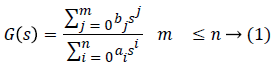
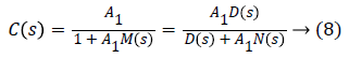
Where C (s) is the transfer function of the controller and M (s) is the model of the process. The method is represented by the transfer function G (s) connecting its signal of control, d (s) is an unmeasured disturbance on the output of the process.
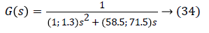
The transfer function for the process G (s) with is considered as:
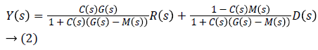
The expression of the output as a function of the set point and the disturbance is expressed by the Equation 2:
Relative to the difficulty to realize the inversion of a dynamic system, the approximated inversion proposed [10-12] is based on the gain A1 that the controller is expressed as:
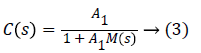
For A1 chosen sufficiently high, C (s) is an approximate inverse of M (s) and consequently C (s) can be used as an IMC regulator.
The structure of the proposed corrector C (s) is given by the following schema (Figure 2).

Figure 2: Structure for model inversion.
Property of the internal model controller
The inversion method for constructing the controller, described by Equations 2 and 3 has the advantage of ensuring the stability, accuracy and speed of the system.
• Static error
If the static gain of the model is M (0), then that of the corrector is equal to:
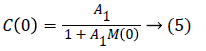
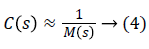
For A1 high enough, Equation 4 becomes:
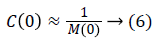
This value given by Equation 5 makes it possible to have a static error of zero.
• Stability
If we ask that the model of the system M (s) is described by the following equation:
Then the transfer function of the controller is given by:
The characteristic equation Ec (s) of C (s) is
The stability of the controller depends on the roots of the equation Ec (s), and is a function of the gain A1. So the value of A1 influence on the stability of the system [12]. The application of the internal model control requires that the system, the model and the controller are stable in open loop to ensure stability, precision and speed in closed loop [10].
Model uncertainty and robust stability analysis
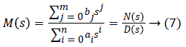
The development of any model of a physical process requires approximations, which therefore introduce model uncertainties. The representation of uncertainties can take different forms; it depends on the nature of the information you want to bring up. Generally, the representation adopted reflects the knowledge of the physical phenomena that cause uncertainty and the ability to represent these uncertainties in a simple and easy to manipulate form [13,14]. The first type of uncertainty is unstructured uncertainty, linked to the existence of a dynamics not represented in the model [15]. The second type, linked to the parametric inaccuracies of the model, directly concerns the modeled part of the dynamics of the system. They can therefore not be adequately treated by unstructured disturbance. An uncertain system with parametric uncertainties at the level of the transfer matrix G (S) of the process is written in the following form:
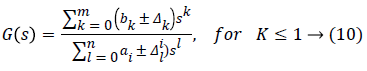
Where Δk and il are the parametric uncertainties of the parameters bk and al respectively, and m and n are respectively the numerator and the denominator of the transfer function G (s).
The uncertain characteristic polynomial of the transfer function G (s) is given by the following equation:
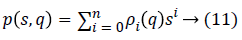
Where q is the vector of uncertainty and ρi are coefficient functions.
The family of polynomials is given by the following Equation 16.
Where Q is the uncertainty.
The family of polynomials 5 is robustly stable if and only if p (s, q) is stable for everyone q ϵ Q.
For the study of the stability of uncertain systems defined by Equation 5, the method of the value set concept and zero exclusion condition seems to be very unique from the viewpoint of its universality and applicability even for the very complex uncertainty structures [16].
Assume a family of polynomials 5. The value set at frequency ω ϵ is given by [15]:
In reality, p (jw, Q) is the image of Q under p (jw,.).
Practical construction of the value sets then means to substitute s for jw, fix w and let the vector of uncertain parameters q range over the set Q.
The zero exclusion condition for Hurwitz stability of family of continuous-time polynomials 2 affirms [16]: suppose invariant degree of polynomials in the family, pathway connected uncertainty bounding set Q, continuous coefficient functions ρi (q) for i=0,1, 2,..., n and at least one stable member p (s, q0). So the family P is robustly stable if and only if the complex plane origin is excluded from the value set p (jw, Q) at all frequencies w ≥ 0, that is P is robustly stable if and only if the Equation 7 is verified:
Presentation of the LVAD System
A left ventricular assist device is placed parallel to the heart and therefore the native heart is left in place [2,17]: blood from the cardiac cavities i.e. the left atrium or ventricular passes through a pump through a tube. Subsequently, the blood is returned to the aorta by another tube as shown in Figure 3.

Figure 3: Left ventricular assist device system.
However, the pouch made in the thickness of the abdominal wall to implant them has complications such as bleeding or infections.
Moreover, the left-ventricular character they have implies that the other side contracts sufficiently to meet the usual needs [17].
The left ventricular assist device is the most common device applied to a defective heart (since it is sufficient in most cases, the right side of the heart is often able to make use of the blood circulation). It should be noted that the ventricular assist device consists essentially of a linear actuator which drives a pump and the latter which makes it possible to pump blood at the apex of the left ventricle and p (jw, Q) returned to the ascending aorta [18].
Motorization of the Left Ventricular Assist Device
The objective of the actuator to be implanted in the aorta is to ensure a physiological pulse flow. For the sake of miniaturization, it is sought with this actuator to obtain both the “valve” function and the “pump” function. In order to validate this principle, we propose to make a linear tubular actuator prototype equipped with a St Jude Medical type unidirectional mechanical valve of 20 mm diameter (Figure 4), which allows the movement of blood.

Figure 4: Basic structure of the prototype actuator.
The linear actuator proposed is a linear switched reluctance actuator consisting of 3 stator coils and a translator (Figure 4). The sequential supply of the coils creates a magnetic field that slides alternately from one to the other end of the actuator by printing the ferromagnetic cylinder back and forth movements. During the translation of the cylinder in one direction, the valve prosthesis closes and exerts pressure on the liquid which allows its training. When translating in the opposite direction, the valve prosthesis opens to limit its effect on the fluid.
The advantages of this type of engine are: its reliability, its simplicity of implementation, its ability to generate a translation movement directly (without mechanical transformation). The main disadvantage lies in the difficulty of guiding the moving part to ensure a constant air gap.
The mechanical characteristics of the actuator
The physiological requirements for an LVAD are a flow rate of 6 l/min and a pressure of 115 mmHg (16 kPa) at a frequency of 120 pulsations per min [17].
By passing to the units of the international system, the physiological parameters of it are reduced and summarized in the following Table 1.
| Physiological parameters | Abbreviation | Value |
|---|---|---|
| Blood flow in the aorta (m3/s) | Q | 9.96.10-5 |
| Arterial pressure (Pa) | P | 15332.03 |
| Cardiac frequency (Hz) | f | 2 |
Table 1. Physiological parameters.
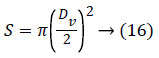
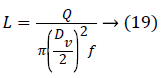
Considering the blood pressure under a valve of diameter Dv=20 mm, the force of the thrust capable of displacing the membrane is given by:
F=PS → (15)
with S is the valve section, she is given by the following equation:
The expression of the pushing force can be reduced to:
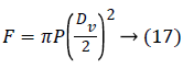
The force of the thrust being 4.82 N and, relative to the incremental actuator operating in open loop, we must then provide a margin of safety on said pushing force by an increase of 25% to avoid stalling [19] in case any elevation of the cardiac pressure. We therefore retain a thrust force of 6.1 N to determine the geometrical parameters of the actuator. The stroke of the actuator is determined by Equation 18.
L=Q/Sf → (18)
By considering Equation 18 of the surface, the equation of the race is reduced to:
Dimensioning of the actuator
The elementary cell (Figure 5) of this actuator consists of a ferromagnetic stator part which comprises two teeth and a notch (with conductors), and a ferromagnetic part of the movable part which itself also comprises two teeth and a notch (without drivers).

Figure 5: Basic structure of the prototype actuator (1/2 cut).
To realize the complete actuator, it is sufficient to stack all the elementary cells by separating them from a non-magnetic part to the stator.
Above shows all the geometrical parameters of the actuator to be determined, Re is the radius of the gap, e the thickness of the air gap, Rext the outer radius of the machine, ec the thickness of the cylinder head, hds the stator tooth height, the height of the translator and c the non-magnetic separation between the different stator modules.
For the motorisation of the left ventricular assist device, we selected the linear incremental actuator with variable reluctance. The latter must be able to generate a thrust force that corresponds to the load force and this on each step of its displacement. It is composed of a cascading succession of three stator modules: 1, 2 and 3; separated by non-magnetic parts. The translator of the actuator is composed of teeth.
Those of the stator module and the notches of the mobile are identical and the same width.
The tooth pitch of the actuator is related to tooth and notch width by the following equation:
λ=a+b → (20)
knowing that a=b
The tooth pitch and the mechanical pitch of the actuator are linked by the following relation:
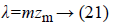
with m=3 (number of phases)
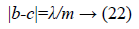
The non-magnetic separation distance c is described by Equation 22.
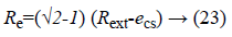
The outer radius of the Rext actuator is to be calculated from the following expression [19].
The length of the stator Lst is given by the following relation:
Lst=mn (2a+b)+c (mn-1) → (24)
with n=1 (one coil per phase)
Width of displacement Lmt
Lmt≥ L+Lst → (25)
Thus, in a summary manner, the geometric parameters of the variable reluctance actuator to be achieved are summarized in Table 2.
| Geometric parameters | Abbreviation | Value (mm) |
|---|---|---|
| Mechanical step | zm | 1.93 |
| Tooth pitch | 5.8 | |
| Tooth width | A | 2.9 |
| Slot width | B | 2.9 |
| Non-magnetic separation | C | 0.97 |
| Stator yoke thickness | ecs | 1.5 |
| Mover yoke thickness | ect | 2 |
| Air gap radius | Re | 13.6 |
| Hauteur de la bobine | hbob | 9.4 |
| Mover tooth lengher | hdt | 1.5 |
| Stator tooth length | hds | 9 |
| Air gap length | e | 0.2 |
| External radius | Rext | 24.2 |
| Valve radius | Rv | 10 |
Table 2. Geometric parameters of the actuator.
Choice and specification of magnetic material
The incremental linear actuator is characterized by two sources of losses: joule losses and iron losses [20]; these losses affect the operating time of the actuator, it is important to consider these losses in the design stage.
On the one hand, joule losses, created in electrical circuits, directly influence the insulating material of the coil [21]. In order to limit the losses generated within the armatures of the magnetic circuits, magnetic alloys are generally used in the form of insulated sheets [22]. The choice of alloys depends on technical and economic aspects. Three families of alloys have penetrated the market for laminated materials: iron-silicon alloys, iron-cobalt alloys and iron-nickel alloys [23,24].
Model of iron losses for magnetic circuits in sheet metal: Iron losses are decomposed into two terms: hysteresis losses and eddy current losses [25]. The formulation of iron losses is governed by the following analytical equation [19-26].
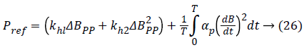
kh1, kh2 and αp representing the ferromagnetic loss coefficients specific to the material used, generally they were determined from data provided by the manufacturers and the total variation of the induction.
Table 3 shows the values of kh1, kh2 and αp for sheet materials, determined or given by the manufacturers [26].
| Material | Thickness of sheet (mm) | Pfer (W/Kg) F=50 Hz Bm=1.5 T | kh1 (A/m) | Kh2 (Am/Vs) | αp (A m/V) |
|---|---|---|---|---|---|
| Fe_Si 3% | 0.5 | 6.5 | 12 | 90 | 0.065 |
| 0.35 | 2.6 | 5 | 40 | 0.022 | |
| 0.1 | 1.72 | 8 | 26 | 0.0028 | |
| Fe_Ni 50-50 | 0.1 | 0.84 | 0 | 14 | 0.0018 |
| Fe_Co 49-49 | 0.1 | 3.65 | 88 | 32 | 0.0015 |
Table 3. Iron loss coefficients for magnetic sheet materials.
The supply voltage of the actuator Un is rectangular in square, corresponds to a triangular induction form B [26], Figure 6; the formulation of iron losses can be simplified to arrive at the following expression [19-26].

Figure 6: Induction form generated by a square-wave voltage.
where f is the frequency associated with the variation of the induction, Bm is the maximum value of the induction and α the inverse of the number of m phases.
Dynamic behavior of the LVAD actuator
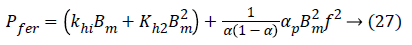
The electrical equations of the linear step actuator considered are given by the following system [19].
The mechanical equation of the linear step actuator considered is given by the following relation [6,19].
In general, the forces F1 (x), F2 (x) and F3 (x) developed by the actuator are sinusoidal knowing that the evolution of the stator inductors is still assumed to be sinusoidal [19]. Therefore, these forces are expressed as follows:
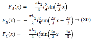
In view of the above, the general equation of motion is finally translated by Equation 31.
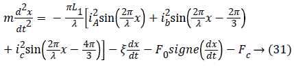
The actuator studied is characterized by the mechanical and electrical parameters summarized in Table 4.
| Electrical and mechanical parameters | Abbreviation | Value |
|---|---|---|
| Mass of the mover (Kg) | m | 1.1 |
| Viscosity coefficient (Nm/s) | Ξ | 65 |
| Static dry friction force (N) | F0 | 1.75 |
| Average value of the Inductance of a phase (H) | L0 | 525.10-5 |
| Amplitude of the inductance of a phase (H) | L1 | 394.10-4 |
| winding resistance (Ω) | R | 8.5 |
| Nominal voltage (V) | Un | 50 |
Table 4. Mechanical and electrical parameters of the actuator.
Figure 7 shows the evolution of the behavior of the currents of three phases IA, IB and Ic. The nominal value of the current is 5.9 A. It is noted that currents with oscillations and overshoots

Figure 7: Variation of position versus time.
Figure 8 shows an oscillatory behavior of the speed of the actuator which requires the insertion of a controller to improve its dynamic performance.

Figure 8: Variation of speed versus time.
Figure 9 shows the evolution of the velocity as a function of the position, it is noted that the central phase is more energetic than the end phases this is mainly due to the effects of extremities.

Figure 9: Variation of speed versus position.
The resolution of the dynamic model described by Equation 31 by applying the Range Kutta algorithm to the order 4 under the Matlab environment makes it possible to determine the evolution of the mobile position x as a function of time t taking into account the load force Fc.
Figure 10 shows the dynamic response of the actuator, angular oscillations appear around the final equilibrium position; these oscillations are derived from the kinetic energy accumulated by the moving part during displacement. The oscillations are damped more or less rapidly by the effects of friction of all kinds, among which we can cite:

Figure 10: Evolution of the dynamic response of position.
- dry friction, viscous friction and part of the iron losses and joules losses associated with the induced motion voltage. These oscillations are unfavorable insofar as precise positioning and without overshoot are required.
Control in Position of LVAD by IMC
By considering the force Fm as the input of the system and the position x as its output and we neglect the friction force; the transfer function of position response can be considered as a typical second-order system following.
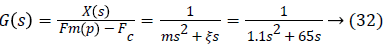
We consider in this part the application of the internal model control in order to suppress the oscillations and exceeding of the dynamic response of the actuator and to cancel the static position error.
The internal model control requires the LVAD system describes by the Equation 32, the model of the system M (s) and the controller C (s) are both stable in open loop.
The model of the system M (s) is chosen to be perfect, so G (s)=M (s).
The poles of the Equation 32 are p1=59.09 and p2=0; therefore the system and the model are at the limit of stability. A gain A1=100 was chosen to ensure the stability of unit response of LVAD in closed-loop. The expression of the internal model controller is given by the following equation.
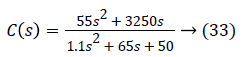
The controller C (s) is stable in open loop because its poles p1'=0.77 and p2 '=58 have a negative real part.
The Figure 11 below shows the dynamic response of the LVAD system subjected to the internal model control, one’s notice that the position of the actuator does not have oscillations. It follows the set point 1.93 mm and stays stable.

Figure 11: IMC of the position of the actuator.
The internal model control can be applied to a microcontroller [27-28].
Robustness of the internal model control
The robustness of the internal model control is to ensure performance and stability of the system face up to disturbances of the environment and also uncertainties model.
Disturbance rejection: The system is subjected to a disturbance of magnitude 10-3 at a period t=10 s. One’s notice that it remains stable, precise and follows the set point and does not exhibit oscillations as shown in Figure 12.

Figure 12: IMC of the position of the actuator with the disturbance.
Uncertainty of parameters: The parameters of the actuator are not exact, so there are uncertainties of the model that must be taken into account to test the robustness of the control strategy used.
Since the mass and viscous friction coefficients are the only two parameters contained in the transfer function of the process, we will therefore calculate their uncertainties by minimizing and maximizing them.
The values of the actuator mass at plus or minus 10% and the viscous coefficient of friction of the latter at plus or minus 5%. Taking into account these uncertainties, the transfer function is written:
It is necessary to study the stability G (s) of the uncertain characteristic polynomial of G (s) to apply the IMC by using the method value set concept and zero exclusion condition.
We see from the Figure 13, the uncertain system does not generate the point (0, 0); then the uncertain system is stable.

Figure 13: Value sets for the characteristic polynomial of G (s).
We see from the Figure 14; the evolution of the position remains devoid of oscillations. The system is stable, precise and follows the fixed set point, which indicates the robustness of the proposed control approach to the fluctuations of the uncertainties in the modeling of the G (s).

Figure 14: IMC of the position of the uncertain parameter actuator
Conclusion
The development of a conventional control technique for increasing the performance and smoothing of the movement of an incremental linear switched reluctance actuator with a tubular structure for the motorization of the left ventricular assist device constitutes the heart of our work searches contained in this article.
Relative to the movement of this actuator studied that is oscillating and exhibits a considerable exceeding, we have here developed the internal model control by its robustness in order to guarantee its precision of positioning. This solution that can be applied in a closed loop, has allowed the smoothing of its movement and the damping of these oscillations.
However, the actuations realized by the actuator studied have been very satisfactory in so far as the results obtained are very coherent, that is say the continuation of the reference which is none other than the mechanical step is indeed ensured, in the absence as well as in the presence of the loading force with a very minimal response time (parameter that is always sought to be minimized for such a device that will be implanted in the human organism).
References
- Blitz A, Fang JC. Ventricular assist devices and total artificial hearts. Contemp Cardiol Dev Ther Heart Fail 2009; 339-371.
- Leprince P. Conception et modélisation dactionneurs électroactifs innovants pour lassistance circulatoire. Ph.D. dissertation, Institut Polytechnique de Toulouse 2005.
- Smith PA, Wang Y, Metcalfe RW, Sampaio LC, Timms DL, Cohn WE, Frazier O. Preliminary design of the internal geometry in a minimally invasive left ventricular assist device under pulsatile-flow conditions. Int J Artific Organs 2018; 41: 144-151.
- Doughty RN. The survival of patients with heart failure with preserved or reduced left ventricular ejection fraction-an individual patient data meta-analysis. Eur Heart J 2012.
- Allen GS, Murray KD, Olsen DB. The importance of pulsatile and non pulsatile flow in the design of blood pumps. Artific Organs 1997; 21: 922-928.
- Jufer M. Electromécanique. Presses Polytechniques et Universitaires Romandes, Lausane 1995.
- Saidi I, El Amraoui L, Benrejeb M. Two-phase switching of a linear step actuator for a syringe pump control. Int Rev Autom Control 2011; 4: 455-460.
- Saidi I, El Amraoui L, Benrejeb M. Electrical syringe pump design using a linear tubular step actuator. Int J Sci Tech Autom Control Comp Eng (IJSTA) 2010; 4: 1388-1401.
- Bejaoui I, Saidi I, Soudani D. New internal model controller design for discrete over-actuated multivariable system. IEEE, 4th International Conference on Control Engeniering and Information Technology (CEIT) Hamamet, Tunisia 2016; 1-6.
- Dhahri A, Saidi I, Soudani D. A new internal model control method for MIMO over-actuated systems. Int J Adv Comp Sci Appl 2016; 7.
- Martinez N, Leprince P, Nogarede B. A novel concept of pulsatile magnetoactive pump for medical circulatory support. Electric Mac ICEM 2008; 1-6.
- Naceur M. Commande par modèle interne des système dynamiques continus et échantillonnés. Ph.D. Dissertation, Ecole Nationale dIngénieurs de Tunis 2008.
- Barmish BR. New tools for robustness of linear systems. Macmillan NY USA 1994.
- Matusu R, Prokop R. Graphical analysis of robust stability for systems with parametric uncertainty: an overview. Trans Inst Measur Control 2011; 33: 274-290.
- Bejaoui I, Saidi I, Soudani D. Internal model control of MIMO discrete under-actuated systems with real parametric uncertainty. International Conference on Advanced Systems and electric Technologie Hammamet, Tunisia 2018.
- Matusu R, Prokop R. Graphical analysis of robust stability for polynomials with uncertain coefficients in Matlab environment. Rec Res Circ Sys 2011; 242-247.
- Bocquillon L. Facteurs pronostiques hémodynamiques pré-opératoires de défaillance ventriculaire droiteaprès implantation de Heart Mate II-étude observationnelle monocentrique. Ph.D. dissertation, Université de Toulouse III-Paul SABATIER 2015.
- Teuteberg JJ, Slaughter MS, Rogers JG, McGee EC, Pagani FD, Gordon R, Rame E, Acker M, Kormos RL, Salerno C, Schleeter TP, Goldstein DJ, Shin J, Starling RC, Wozniak T, Malik AS, Silvestry S, Ewald GA, Jorde UP, Naka Y, Birks E, Najarian KB, Hathaway DR, Aaronson KD. Advance Trial Investigators. The HVAD left ventricular assist device: risk factors for neurological events and risk mitigation strategies. JACC Heart Fail 2015; 3: 818-828.
- Saidi I. Sur la modélisation multidisciplinaire dun système de motorisation linéaire. Application au cas dun pousse-seringue, Ph.D. dissertation, Ecole Nationale dIngénieurs de Tunis 2011.
- Chevallier S. Comparative study and selection criteria of linear motors. Ph.D. Dissertation, Federal Polytechnic School of Lausanne 2006.
- Maye P. Moteurs électriques pour la robotique. Electrotechnique, Edition Dunod, Paris 2000.
- Cyr C. Modélisation et caractérisation des matériaux magnétiques composites doux utilisés dans les machines électriques. Ph.D. dissertation, Faculté des Etudes Supérieures de lUniversité de Laval Québec 2007.
- Alhassoun Y. Alhassoun Etude et mise en œuvre de m achines à aimantation induite fonctionnant à haute vitesse. Ph.D. dissertation, Institut National Polytechnique de Toulouse 2005.
- Duhayon E, Henaux C, alhassoun Y, Nogarede B. Design of a high speed switched reluctance generator for aircraft applications. 15th ICEM, Bruge 2002.
- Bertotti G. General properties of power losses in soft ferromagnetic materials. IEEE Trans Magn 1988; 24: 621-630.
- Hoang E. Etude, modélisation et mesure des pertesmagnétiques dans les moteurs à réluctance variable à double saillanc es. Ph.D. Dissertation, ENS Cachan 1995.
- Chuen Gan W, Cheung NC, Qiu L. Position control of linear switched reluctance motors for high precision applications. IEEE Trans Industry Appl 2003; 39.
- Mamun AL, Ahmed N, Alqahtani M, Altwijri O, Rahman M, Ahamed NU, Rahman SAMM, Ahmad RB, Sundaraj KKK. A microntroller-based automatic heart rate counting system from finger TIP. J Theor Appl Info Technol 2014; 62.