Research Article - Biomedical Research (2017) Volume 28, Issue 11
Computational intelligence-based decision support system for glaucoma detection
Karkuzhali S* and Manimegalai D
Department of Information Technology, National Engineering College, Kovilpatti, Tamil Nadu, India
- *Corresponding Author:
- Karkuzhali S
Department of Information Technology, National Engineering College, Tamil Nadu, India
Accepted date: March 11, 2017
Abstract
Glaucoma is the second major cause of loss of vision in the world. Assessment of Optic Nerve Head (ONH) is very important for diagnosing glaucoma and for patient monitoring after diagnosis. Robust and effective Optic Disc (OD), Optic Cup (OC) detection is a necessary preprocessing step to calculate the Cup-To-Disc Ratio (CDR), Inferior Superior Nasal Temporal (ISNT) ratio and distance between optic disc center and optic nerve head (DOO). OD is detected using Region Matching (RM) followed by medial axis detection in fundus images. OD and OC segmentations are carried out by Improved Super Pixel Classification (ISPC), Adaptive Mathematical Morphology (AMM) and the effectiveness of the algorithm is compared with existing k-means and fuzzy C means (FCM) algorithm. Experiments show that OD detection accuracies of 100%, 98.88%, 98.88% and 100% are obtained for the DRIVE, DIARETDB0, DIARETDB1 and DRISHTI data sets, respectively. In this work, three statistically significant (p<0.0001) features are used for Naive Bayes (NB), k-Nearest Neighbor (k-NN), Support Vector Machine (SVM), Feed Forward Back Propagation Neural Networks (FFBPNN), Distributed Time Delay Neural Network (DTDNN), radial basis function exact fit (RBFEF) and Radial Basis Function Few Neurons (RBFFN) classifier to select the best classifier. It is demonstrated that an average classification accuracy of 100%, sensitivity of 100%, specificity of 100% and precision of 100% have been achieved using FFBPNN, DTDNN, RBFEF and RBFFN. With expert ophthalmologist's validation, Decision Support System (DSS) used to make glaucoma diagnosis faster during the screening of normal/ glaucoma retinal images.
Keywords
Glaucoma, Retina, Optic disc, Optic cup, Cup to disc ratio, ISNT ratio.
Introduction
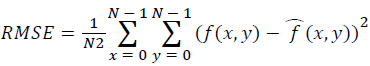
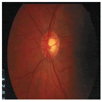
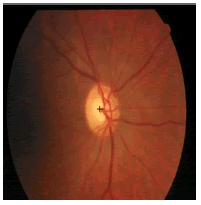
Glaucoma is a degenerative eye disease, in which the optic nerve is gradually damaged due to increased pressure causing loss of vision and eventually to a state of irreversible blindness [1]. According to World Health Organization, glaucoma is the second prime leading cause of blindness in the world [2]. The widespread model estimates that about 11.1 million people worldwide will suffer from glaucoma-induced irreversible blindness in 2020 [3]. Eye pressure occurs due to blockage in trabecular meshwork when aqueous humor flows in anterior chamber in the front part of our eye, plays a role in damaging the delegate nerve fibers of the optic nerve. Raised pressure inside the eye is called Intra Ocular Pressure (IOP) which has normal IOP of ~10 mmHg and glaucoma IOP>20 mmHg, even patients with normal pressure can have glaucoma [4,5]. The design of Decision Support System (DSS) for glaucoma diagnosis depends on image cues and imaging modalities such as Optic Disc (OD) and Optic Cup (OC). OD is an oval brightest region in posterior chamber of the eye where ganglion nerve fibers assemble to form Optic Nerve Head (ONH). The center of OD has white cup-like area called OC [6]. The annular region between OD and OC is called as Neuroretinal Rim (NR). The damage appears in optic nerve fibers leads to a change in the structural manifestation of the OD; the magnification of the OC (thinning of NR) is called cupping [7,8]. Figure 1 shows normal and abnormal retina. It may be mentioned here that glaucoma can be detected by measurement of IOP, visual field analysis and consideration of ONH. Assessment of damaged ONH is more effective and accurate to IOP measurement or visual field testing for glaucoma screening. Automatic ONH assessment plays a vital role in developing DSS for diagnosing glaucoma [9,10].

Figure 1: Diagrammatic representation of normal and glaucomaaffected retina.
OD and OC detection is based on the detailed analysis of digital fundus images. In the diagnosis of glaucoma, considerable study has been carried out to find OD and OC in fundus images. There have been a number of reports available on color retinal images for detection of OD and OC [11-24]. The detection of glaucoma begins with preprocessing the retinal image, and localization of OD, which are followed by segmentation of OD and OC. The OD localization is carried out by Hough transformation [11] and Fourier transformation and p-tile for thresholding [12]. OD and OC segmentations by combination of Hough transform [12,13] and Active Contours Model (ACM) [12] have been reported. At the same time OD and OC boundary detection by active snake model and active shape model [13] is also carried out. OD localization is done by illumination modification and boundary segmentation by a Supervised Gradient Vector Flow snake (SGVF) model [14]. OD localization and segmentation using template matching and level set method [15] are also implemented.
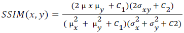
The localization of OD is carried out by selecting the significant scale-space blobs [16], and at the same time OD can be segmented by extracting the features such as compactness, entropy and blob brightness [16]. Comparison of OD segmentation algorithms such as ACM, fuzzy C means (FCM), and Artificial Neural Networks (ANN) has been reported [17]. A line operator has been used to capture circular brightness structure of OD [18]. However, a circular transformation is used to mark rounded contour and image dissimilarity across the OD [19]. Automated localization of the OD in color eye fundus images, has been extracted from the blood vessels with intensity data [20] and adaptive morphological two-stage approach [21]. The localization of OD has been performed using fast radial transform and vessel density estimation [22]. Interestingly, OC is segmented using multi-scale super pixel segmentation, and the boundary is detected using ellipse fitting algorithm [23]. Alternatively, OC can be segmented using motion boundary and its boundary by best circle fitting [24]. In the present investigation, a DSS system has been developed for detection of glaucoma using three clinical indicators such as Cup-to-Disc Ratio (CDR), Inferior Superior Nasal Temporal (ISNT) Ratio and distance between optic disc center and optic nerve head (DOO). CDR compares area of OC with area of OD. ISNT ratio is the relation between total area of vascular network in inferior and superior side of the OD to the total area of the vascular network in nasal and temporal areas [10]. Figure 2 shows the major structural indicators of glaucoma.

Figure 2: Diagrammatic representation of (a) CDR, (b) ISNT ratio for normal and abnormal retina (c) Distance between OD center and ONH.
An attempt has been made to localize OD using Region Matching (RM). Subsequently, OD and OC segmentations have been carried out using Improved Super Pixel Classification (ISPC), Adaptive Mathematical Morphology (AMM) approach, k-means and FCM followed by feature vector formation and glaucoma classification by Naive Bayes (NB), k-NN (k-Nearest Neighbor), Support Vector Machine (SVM), Feed Forward Back Propagation Neural Networks (FFBPNN), Distributed Time Delay Neural Network (DTDNN), Radial Basis Function Exact Fit (RBFEF) and Radial Basis Function Few Neurons (RBFFN).
Materials and Methods
An attempt has been made here to develop a DSS to diagnose glaucoma. The assessment of ONH is carried by extracting image features for binary classification of healthy and glaucomatous subjects. During the assessment, the OD localization is an important preprocessing stage since it helps to localize and segment OD and OC to evaluate CDR, ISNT ratio and DOO. The localization of OD is carried out by preprocessing the input image and reference retinal image. The first step of preprocessing is to convert RGB to HSV image. Then, histogram equalization and histogram matching are applied in both the images to reduce uneven illuminations. The localization of OD is carried out using RM and k-NN search by Kd-trees; on the other hand the detection of OD centre is by medial axis (Scheme 1).

Scheme 1: Flow diagram of the proposed approach.
In the segmentation of OD, Simple Linear Iterative Clustering (SLIC) is employed to aggregate pixels to super pixels. Further, the features like histograms and Center Surround Statistics (CSS) are extracted to classify each super pixel as OD or non-OD by SVM classifier. In order to compare the efficiency and accuracy of OD segmentation, AMM approach, k-means and FCM algorithms are used. Similarly, OC is also segmented by following the methodology adopted in segmentation of OD. Subsequently, the feature extraction is done by calculating CDR, ISNT ratio and DOO. Then, feature vector is formed using these three prime factors and given as an input for image classification and pattern recognition tasks (Scheme 1).
Image acquisition
Drishti-GS data set (http://cvit.iiit.ac.in/projects/mip/drishti-gs/ mip-dataset2/Home.php) consists of 101 images were collected from Aravind Eye Hospital, Madurai. The patients were between 40-80 years of age and OD centered images with dimensions of 2896 × 1944 pixels. Expert annotated images were collected from ophthalmologist with clinical experience of 3, 5, 9 and 20 years [25].
OD Localization using region match
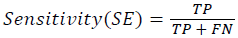
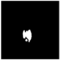
Before processing the retinal images for localization of OD, it is necessary to preprocess the retinal images to handle the illumination variations caused due to image acquisition under various conditions. Adaptive histogram equalization is used as preprocessing step to localize OD. Further, the RGB image is converted to grayscale. The histogram matching is performed between the cropped image (CI) and the Original Image (OI), and then the image is converted to HSV color space. In CI and OI, the correspondence map for every block is computed by block distance metric such as Euclidean distance. In RM, every block is approximated to a low dimensional feature, and these are used to find the nearest neighbor. The RM is computed by the following sequence: calculate the mean of R, G, B channels in the color fundus image, mean of X, Y gradients of the block, frequency components (first 2) of Walsh Hadamard Kernels and then finally the maximum value of the block.
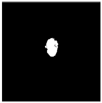
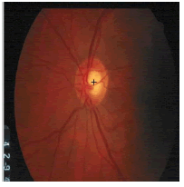
The k-NN search has been performed effectively for low dimensional data using different categories of tree structures [8]. Construction of Kd-tree is done by the node points are iteratively partitioned into two sets at each node and by splitting along one dimension of the data until one of the termination criteria is met. Adaptive thresholding is used to segment OD. The OD is located by calculating the row center and column center by taking the average between the minimum number of rows/columns and the maximum number of rows/ columns. The intersection point of row center and column center is marked as the OD center. Figure 3 shows the localization of OD using RM.

Figure 3: Sample results of localization of OD using RM.
OD segmentation and OC segmentation
Improved super pixel classification: The segmentation of OD is performed using ISPC. The SLIC algorithm is used to group neighborhood pixels into super pixels in retinal fundus images. Histogram and CSS are used to classify each pixel as OD or non-OD in the segmentation of OD. It is worth mentioning that classification is performed using SVM. The output value is used as the assessment values for all pixels in the super pixel. Further, smoothed assessment values are used to obtain binary assessment values. Finally, +1, -1 and 0 are assigned to OD, non-OD and threshold respectively. Likewise, the resultant matrix with 1's and 0's is designated as OD and Non-OD (background) respectively [9].
The following steps elaborately describe the ISPC for OD and OC segmentation.
Step 1: Compute SLIC by S=vT/D where T is the total number of super pixels, D is desired number of super pixels
Step 2: Compute histogram equalization for r, g, b from RGB color space and h, s from HSV color space HISTj=(HISTr HISTg HISTb HISTh HISTs). The histogram computation counts number of pixels in 256 scales for R, G, B, H, and S to get 1280 dimensional features.
Step 3: Generate nine spatial scales dyadic Gaussian pyramids with a ratio from scale zero (1:1) to scale eight (1:256).
Step 4: Accomplish Low Pass Filter (LPF) version of Gaussian pyramid by convolution with separable Gaussian filter and decimation by factor 2.
Step 5: Compute CSS features as the mean and the variance of the maps within the super pixels.
Step 6: Expand CSS feature for SPj to CSSj=(CSSj CSSj1 CSSj2 CSSj3 CSSj4). It has a dimension of 18 × 2 × 5=180.
Step 7: Combine the final feature (HISTOD, CSSOD) and (HISTOC, CSSOC).
Step 8: Assign output value for each super pixel as the assessment values for all pixels.
Step 9: Obtain the binary decisions for all pixels by smoothing decision values with a threshold.
Step 10: Assign +1 and -1 to OD and non-OD samples, and the threshold is the average of them, i.e. 0. 1 as OD and 0 as background.
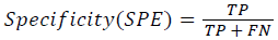
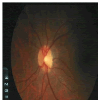
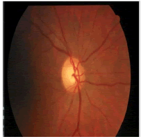
Adaptive mathematical morphology (AMM): AMM is a non-linear image processing methodology and extracting ideas from set theory, topology and discrete mathematics. It is based on minimum (erosion) and maximum (dilation) operators whose aim is to extract the significant structures of an image with thresholding operation. The segmentation of OD and OC is carried out using combination of morphological operations and adaptive thresholding. Figure 4 shows results of ISPC and AMM. k-means and FCM algorithm performed using the steps carried out in our previous work [26].

Figure 4: Sample results show segmentation of OD and OC using ISPC and AMM.
The following steps describe clearly the sequence of morphological operations.
Step 1: Perform close and open operation in R and G components
Close-Fill the holes in lightest region both OD and OC region
Open-Remove any small light spots
Step 2: Separate disc and cup with standard deviation (SD) and Threshold value
R component-Threshold=SD × 3.2
G component-Threshold=SD × 4.0
Step 3: Calculate OD and OC area by adding the number of white pixels
Step 4: Detect OD center in cropped green channel image by thresholding
Step 5: Identify ONH coordinates by finding area of lightest intensity in bottom hat transformed OD cropped image
Step 6: Compute Euclidean distance between 2 points as distance between OD center and ONH
Step 7: Crop binary image of blood vessel to 300 × 300
Step 8: Generate 300 × 300 masks to cover 1 quadrant, rotated to 90 deg. each time to generate 4 masks
Step 9: Compute ISNT ratio by relation between area of vascular network enclosed by inferior and superior region to area of vascular network enclosed by nasal and temporal region of the cropped OD [10].
Feature vector formation
The feature vector can be formed using three prime parameters as shown below [10]:
CDR: Cup-to-Disc Area Ratio (CAR)=OC area/OD area. (CDR>0.3 indicates the high risk of glaucoma)
ISNT ratio: ISNT ratio=Sum of vascular network area in inferior and superior regions/area of vascular network in nasal and temporal regions [10]. (Lower ISNT ratio increases the risk of presence of glaucoma). Glaucoma damages superior and inferior first and then temporal and nasal optic nerve fibers, and it leads to decrease the area of vascular network in superior and inferior NR rim and change the order of ISNT (I S N T) relationship. Early diagnose of glaucoma was performed successfully by the detection of NR rim distances in inferior, superior, nasal and temporal directions to validate ISNT rule [27].
Distance between ONH and OD center (DOO):
• The ONH coordinates are identified by locating the area of lightest intensity in OD cropped bottom hat transformed image.
• Similarly, the OD center is also detected by recognizing the area of pixels with lightest intensity.
• The Euclidean distance between OD center and ONH is computed to detect DOO. DOO is high for normal eye.
Glaucoma classification
In the present work, seven classifiers, namely NB [3], k-NN, SVM [3], FFBPNN [10], DTDNN [28], RBFEF [28] and RBFFN have been employed to classify glaucoma. The retinal images are classified as normal or glaucoma using appropriate tools based on its features. The images marked as normal or abnormal with the aid of k-NN, SVM, NB, neural network tools available in MATLAB software. The glaucoma affected retinal images are classified using the statistically significant features such as CDR (<0.3, ?0.3), ISNT rule (high/low) and DOO (high/low). By using k-NN classifier, a trained set, a sample set and a group are created. Based on the trained set, the samples are classified into normal and glaucoma cases [25]. In SVM classifier, v-SVM is used with penalization parameter v=0.5 and cost parameter c=1 [3]. Feed forward back propagation neural networks (FFBPNN), Distributed timedelay neural network (DTDNN), Radial basis function exact fit (RBFEF), Radial basis function few neurons RBFFN contains three layers, which are input, hidden and output layer. Three nodes for input layer, hidden neurons are set as 6, and output layer has 2 nodes which are normal and abnormal. RBFEF used for exact interpolation of data in multidimensional space and RBFFN used to achieve good accuracy with interpolation of few neurons [28]. There are three features are applied to the input layer for 26 images (13 is normal, 13 is abnormal) and the targets are set as normal and abnormal.
Results and Discussion
In the present investigation, DRISHTI database with 101 images are used. Among the 101 images, 31 are normal and 70 are glaucoma cases. It is observed that ISPC algorithm is highly suitable for further processing. The statistical significance of features is analysed using student t-test. The outcome of the statistical test of the extracted features is shown in Table 1. It is clearly observed that, the features are statistically significant (p<0.0001).
| Features | Normal (Mean ± SD) | Glaucoma (Mean ± SD) | P value |
|---|---|---|---|
| CDR | 0.1942 0.0574 | 0.7539 0.1066 | <0.0001 |
| ISNT ratio | 3.227 0.3617 | 1.120 0.4632 | <0.0001 |
| DOO | 5553.00 511.53 | 1079 122.36 | <0.0001 |
Table 1: Summary statistics of features used for normal and glaucoma groups.
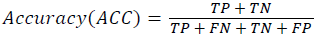
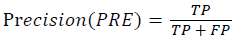
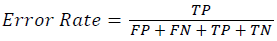
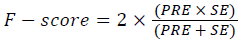
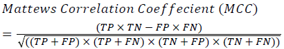
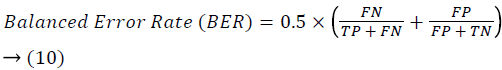
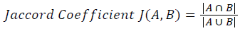
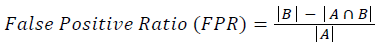
Training and testing set contains retinal images which are completely different and no overlapping found between them. To evaluate the performance of segmentation algorithms compared output of segmentation algorithm with expert annotated images. The performance evaluations for localization of OD are measured using Root Mean Square Error (RMSE), Structural Similarity Index Measure (SSIM) Equations 3 and 4 and for segmentation of OD are measured using sensitivity (SE), specificity (SPE), Accuracy (ACC), Precision (PRE), Error Rate (ER), f-score, classification accuracy (CA), Matthews Correlation Coefficient (MCC), Balanced Error Rate (BER), Misclassified Proportion (MP), Jaccord Coefficient (JC), Dice Coefficient (DC), False Positive Ratio (FPR), False Negative Ratio (FNR) Equations 1-9.
 →(1)
→(1)
 →(2)
→(2)
 →(3)
→(3)
 →(4)
→(4)
 →(5)
→(5)
 →(6)
→(6)
 →(7)
→(7)
 →(8)
→(8)
Classification Accuracy (CA)=The probability (%) that the classifier has labeled an image pixel into the expert annotated class and its being correctly classified as such.
 →(9)
→(9)
 →(10)
→(10)
 →(11)
→(11)
 →(12)
→(12)
 →(13)
→(13)
 →(14)
→(14)
 →(15)
→(15)
Where, f (x, y),f ?(x, y) Equation 6 μx, μy, σx2, σy2, C1, C2. Equation 7 TP, TN, FP, FN (Equations 12-16), A and B (Equations 10-15) are average differences between original image and segmented image, mean and covariance of segmented image and ground truth image, constants (C1 and C2), true positive, true negative, false positive, and false negative, segmented image and ground truth image respectively. If expert annotated image and segmented output are positive as positive and negative as negative, then it will be TP and TN respectively. If expert annotated image and segmented output are negative as positive and positive as negative, then it will be FP and FN respectively. With respect to this statistical treatment, SE is defined as the percentage of unhealthy image in expert annotation is classified as unhealthy in segmented output. SPE defined as the percentage of healthy image in expert annotation is classified as healthy in segmented output.
Tables 2 and 3 present the experimental results obtained by the OD localization and segmentation algorithm, which reveals that the algorithm yields hopeful results in terms of RMSE, SSIM, SE, SPE, ACC and PRE even though only low-quality images are used as test images. Average of the Equations 8-20 was calculated for all images in the data set to obtain the overall performance measure (Table 3). Among the 101 images employed, 50 images are used for training and the remaining 51 images are used for testing. In the present work, out of the 51 images used for testing, 26 (13 are normal, 13 are glaucoma affected) images are used for evaluation. The FFBPNN, DTDNN, RBFEF and RBFFN classifier is used to classify 13 glaucoma-affected images as glaucoma and 13 normal images as normal. It is observed that the average classification rate is 100%, which is clinically significant.
| Image ID | Original image | Segmented OD | Localized OD | SSIM | RMSE |
|---|---|---|---|---|---|
 |
 |
 |
0.7143 | 0.0568 | |
 |
 |
 |
0.7052 | 0.0589 | |
 |
 |
 |
0.703 | 0.0534 |
Table 2: Performance of the proposed localization algorithm.
| Algorithm | OD Segmentation | OC Segmentation | ||||||
|---|---|---|---|---|---|---|---|---|
| Performance measures | ISPC | AMM | K means algorithm | FCM | ISPC | AMM | K means algorithm | FCM |
| Sensitivity (%) | 97.17 | 94.44 | 96.23 | 97 | 94.56 | 88.61 | 88.91 | 93.41 |
| Specificity (%) | 95.87 | 84.74 | 91.27 | 85.43 | 93.65 | 82.59 | 82.44 | 83.26 |
| Accuracy (%) | 97.23 | 93.42 | 93.45 | 94.36 | 98.42 | 94.56 | 88.52 | 92.65 |
| Precision (%) | 99.999 | 99.991 | 99.99 | 99.994 | 99.996 | 99.996 | 99.993 | 99.993 |
| Error rate | 0.0212 | 0.0118 | 0.0116 | 0.0186 | 0.0157 | 0.0133 | 0.007 | 0.0063 |
| F score (%) | 99.989 | 99.994 | 99.994 | 99.99 | 99.9921 | 99.9933 | 99.9965 | 99.9969 |
| Classification Accuracy (%) | 99 | 99.34 | 97.84 | 99.16 | 98.072 | 98.388 | 98.353 | 98.307 |
| Mathews Correlation Coefficient | 0.8134 | -0.0054 | -0.5 | 0.15285 | 0.7483 | 0.1636 | 0.0004 | 0.0002 |
| Balanced error rate | 0.3637 | 0.5 | 0.5 | 0.3948 | 0.5 | 0.375 | 0.5 | 0.5 |
| Misclassified Proportion | 0.00003 | 0.0086 | 0.00908 | 0.00594 | 0.0003 | 0.00354 | 0.00703 | 0.00626 |
| Jaccord coefficient | 0.92304 | 0.8896 | 0.37382 | 0.8378 | 0.74896 | 0.6917 | 0.3149 | 0.37049 |
| Dice coefficient | 0.00402 | 0.00395 | 0.00327 | 0.0072 | 0.00393 | 0.0036 | 0.0032 | 0.00363 |
| False positive rate | 0.97915 | 0.92467 | 0.00341 | 0.00137 | 0.81433 | 0.73954 | 0.00032 | 0.0014 |
| False negativerate | 0.996 | 0.9961 | 0.9984 | 0.9964 | 0.99642 | 0.99684 | 0.984 | 0.9982 |
Table 3: Performance of the proposed OD and OC segmentation algorithm.
Table 4 shows SE, SPE, ACC and PRE for the normal and glaucoma cases using seven classifiers. The FFBPNN, DTDNN, RBFEF and RBFFN classifier is able to detect abnormality with an SE of 100%, an SPE of 100% and PRE of 100%. Tables 5-7 show the comparison of OD localization and OD and OC segmentations algorithms for the present investigation with the reported results. Table 8 shows the tuning parameters for neural networks classifier. It is clearly seen from Table 5 that the RM algorithm for OD localization is highly suitable for DRIVE and DRISHTI database [29-36]. It may be mentioned here that many of the reports have used only CDR-ISNT ratio for the extraction of features [27,37-45], whereas in the present work, in addition to CDR-ISNT ratio, DOO is also computed. The segmentation of OD and OC requires computation time of 6.4s and 1.3s respectively. It is clearly seen from Table 6 that much less computation time is required in the present work than the results already reported by Cheng et al. [9]. It is also confirmed that much less overlapping error (2.12% for OD and 1.57% for OC) is observed than the report by Cheng et al. [9] (9.5% for OD and 24.1% for OC) and Yin et al. [41] (9.72% for OD and 32% for OC).
| Algorithm | TP | FN | TN | FP | SE | SPE | ACC | PRE |
|---|---|---|---|---|---|---|---|---|
| k-NN Classifier | 13 | 0 | 12 | 1 | 100 | 92.3 | 96.15 | 92.85 |
| Naive Bayes | 11 | 0 | 13 | 2 | 100 | 86.66 | 92.3 | 100 |
| SVM | 12 | 0 | 13 | 1 | 100 | 92.85 | 96.15 | 100 |
| FFBPNN | 13 | 0 | 13 | 0 | 100 | 100 | 100 | 100 |
| DTDNN | 13 | 0 | 13 | 0 | 100 | 100 | 100 | 100 |
| RBFEF | 13 | 0 | 13 | 0 | 100 | 100 | 100 | 100 |
| RBFFN | 13 | 0 | 13 | 0 | 100 | 100 | 100 | 100 |
Table 4: Performance of classification algorithm.
| Author name | Year | Ref | Algorithm | Database | Number of images | Computational time(s) | Accuracy (%) |
|---|---|---|---|---|---|---|---|
| Youssif et al. | 2008 | [29] | Vessel direction matched filter | STARE | 81 | - | 98.77 |
| DRIVE | 40 | 100 | |||||
| Niemeijer et al. | 2009 | [30] | Position regression based template matching | Local Database | 1100 | 7.6 | 99.4 |
| Aquino et al. | 2010 | [31] | New template-based method | Messidor | 1200 | 1.67 | 99 |
| Welfer et al. | 2010 | [32] | Adaptive morphological approach | DRIVE | 40 | 100 | |
| DIARETDB1 | 89 | 7.89 | 97.75 | ||||
| Mahfouz et al. | 2010 | [33] | Projection of image features | STARE | 81 | 0.46 | 92.6 |
| DRIVE | 40 | 0.32 | 100 | ||||
| DIARETDB0 | 130 | 0.98 | 98.5 | ||||
| DIARETDB1 | 89 | 0.98 | 97.8 | ||||
| STARE | 81 | 99.75 | |||||
| Lu et al. | 2011 | [19] | Circular transformation | ARIA | 120 | 5 | 97.5 |
| Messidor | 1200 | 98.77 | |||||
| Yu et al. | 2012 | [15] | Directional matched filter | Messidor | 1200 | 4.7 | 99 |
| Zubair et al. | 2013 | [34] | High intensity value of OD | Messidor | 1200 | - | 98.65 |
| Saleh et al. | 2014 | [35] | Fast fourier transform-based template matching | DRIVE | 40 | - | 100 |
| Yu et al. | 2015 | [36] | Morphological and vessel convergence approach | DRIVE | 40 | - | 100 |
| DIARETDB1 | 89 | 99.88 | |||||
| Messidor | 1200 | - | 99.67 | ||||
| Proposed method | Region Matching algorithm | DRIVE | 40 | 100 | |||
| DIARETDB0 | 130 | 98.88 | |||||
| DIARETDB1 | 89 | 98.88 | |||||
| DRISHTI | 101 | 100 | |||||
Table 5: OD localization results for the proposed and literature reviewed methods.
| Author | Image processing Technique | Year | Feature extracted | Database | Number of images | SE(%) | SPE(%) | Overlap error (%) | Success rate (%) | Computation time (s) | Ref |
|---|---|---|---|---|---|---|---|---|---|---|---|
| Wong et al. | Variational level set approach and ellipse fitting | 2008 | CDR | Singapore Malay Eye Study(SiMES) | 104 | 4.81 | [37] | ||||
| Wong et al. | Level set segmentation and Kink based method | 2009 | CDR | Singapore Eye Research Institute(SERI) | 27 | 81.3 | 45.5 | [38] | |||
| Narasimhan et al. | K-Mean clustering and local entropy thresholding | 2011 | CDR-ISNT ratio | Aravind Eye Hospital(AEH) | 36 | 95 | [38] | ||||
| Ho et al. | Vessel inpainting, circle fitting algorithm and active contour model(ACM) | 2011 | CDR-ISNT ratio | Chinese Medical University Hospital | [39] | ||||||
| Mishra et al. | Multi-thresholding, ACM | 2011 | CDR | UK OD organization Messidor | 25, 400 | [40] | |||||
| Yin et al. | Model-based method and Knowledge-based circular Hough transform | 2012 | Distance measure | ORIGA | 650 | 9.72 (OD), 32 (OC) | [41] | ||||
| Narasimhan et al. | k-means and ellipse fitting | 2012 | CDR-ISNT ratio | AEH | 50 | [42] | |||||
| Damon et al. | Vessel Kinking | 2012 | SERI | 67 | [43] | ||||||
| Cheng et al. | Super pixel algorithm | 2013 | CDR | SiMES Singapore Chinese Eye Study (SCES) | 650, 1676 | 9.5, 24.1 | 10.9 (OD), 2.6 (OC) | [9] | |||
| Annu et al. | Wavelet energy features | 2013 | Energy | Local database | 20 | 100 | 90 | 95 | [44] | ||
| Chandrika et al. | K means pixel clustering & Gabor wavelet transform | 2013 | CDR Texture | [45] | |||||||
| Ingle et al. | Gradient method | 2013 | [47] | ||||||||
| Cheng et al. | Sparse dissimilarity constraint | 2015 | CDR | SiMES,SCES | 650, 1676 | [48] | |||||
| Proposed method | ISPC | CDR,ISNT ratio, DOO | DRISHTI | 101 | 97.17, 94.56 | 95.87, 93.65 | 2.121.57 | 97.23, 98.42 | 6.4, 1.3 |
Table 6: Results for segmentation of OD and OC for the proposed and literature reviewed methods.
| Author | Image processing Technique | Year | Feature extracted | Database | Number of images | SE (%) | SPE (%) | Overlap error (%) | Success rate (%) | Computation time (s) | Ref |
|---|---|---|---|---|---|---|---|---|---|---|---|
| Acharya et al. | SVM, Sequential minimal optimization, NB, random forest | 2011 | Texture, Higher order spectra (HOS) features | Kasturba medical college, Manipal | 60 | - | - | - | 91 | - | [49] |
| Acharya et al. | Gabor transformation | 2015 | Mean, variance, skewness, Kurtosis, energy, shannon, Renyi, Kapoor entropy | Kasturba medical college, Manipal | 510 | 89.75 | 96.2 | - | 93.1 | - | [50] |
| Principal component analysis | |||||||||||
| Kolar et al. | Fractal dimension, SVM | 2008 | - | Own database | 30 | - | - | - | - | - | [51] |
| Mookiah et al. | SVM polynomial 1, 2, 3 & RBF | 2012 | HOS, discrete wavelet transform (DWT) | Kasturba medical college, Manipal | 60 | 93.33 | 96.67 | - | 95 | - | [52] |
| Nayak et al. | Mathematical morphology and thresholding, Neural networks | 2009 | Cup-to-disc ratio, ISNT ratio, distance between OD center to ONH to diameter of OD | Kasturba medical college, Manipal | 61 | 100 | 80 | - | - | - | [10] |
| Noronha et al. | Linear discriminate analysis, SVM, NB | 2014 | HOS | Kasturba medical college, Manipal | 272 | 100 | 92 | -- | 84.72 92.65 |
- | [53] |
Table 7: Results for segmentation of OD and OC for the proposed and literature reviewed methods.
| Normal/Abnormal | Image | Classification output | |||
|---|---|---|---|---|---|
| FFBPNN | DTDNN | RBFEF | RBFFN | ||
| Normal | 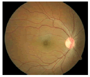 |
0.9999 | 1 | 1 | 1 |
| Abnormal | 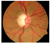 |
0.00085136 | 0.00004816 | 0.00001384 | 0.00001632 |
Table 8: Tuning parameters of neural network classifiers.
Extracting energy features obtained using 2D discrete wavelet transform subjects these signatures to various feature extraction and feature ranking methodologies. Five different classifiers such as LIBSVM, Sequential minimal optimization_1 (SMO_1), SMO_2, Random Forest, NB are used for classification and they showed a ACC, PRE, SE, SPE of {100% 100% 100% 100%}, {100% 100% 100% 100%}, {88.29% 81.82% 100% 100%} and {100% 100% 100% 100%} values respectively [3]. The localization of OD is performed using sliding window, a new histogram-based feature in machine learning framework. The support vector regression-based on RBF is used for feature ranking and nonmaximal suppression for decision- making. The method is tested on ORIGA database, and achieved overlapping error, CDR error and Absolute area difference are 73.2%, 0.09 and 31.5 respectively [6]. Region growing with Active Contour Model (ACM) and vessel bend detection followed by 2D spline interpolation are used for segmentation of OD and boundary of OC. The method has been evaluated on 138 retinal images. They minimize estimation error for vertical CDR, CAR are 0.09/0.08 and 0.12/010 respectively [7]. The segmentation of OD and OC by SPC is followed by selfassessment reliability score and achieved average overlapping error 9.5% and 24.1% respectively. The method is evaluated with 650 images from two data sets and achieved area under curve 0.800 and 0.822 for them [9].
The mathematical morphology followed by thresholding is used for segmentation of OD, OC, blood vessels and ANN for classification of glaucomatous images. This method is able to distinguish normal and glaucoma classes with an SE of 100% and SPE of 80% respectively [10]. Measurement of displacement of blood vessel within OD caused by the growth of OC is the prime factor for the assessment of glaucoma. Their system yielded an SE of 93.02%, SPE of 91.66%, AUC of 92.3% and accuracy of 92.34% [12]. Localization and segmentation of OD and OD boundary are carried out by illumination correction and SGVF snake model with overall performance of 95% and 91% respectively [14]. Segmentation and localization of OD are performed by region, local gradient information and template matching algorithm. This method yielded a success rate of 99%, and the total distance between result of boundary of segmented image and ground truth is 10% [15]. The decision tree, regression-based classifier and majority voting classifiers used features like compactness, entropy and blob brightness features from scale-space blob for identification of OD in retinal images. Their algorithm demonstrated an SE of 85.37% and PPV of 82.87% in the detection of OD [16]. Segmentation of OD is performed using three methods, namely ACM, FCM, ANN for calculating cup to disc ratio for glaucoma screening. Their system showed overlap measure {0.88, 0.87}, {0.88 0.89} and {0.86, 0.86} for all the images [17]. The designed line operator is used for detection of OD, which is characterized by circular brightness structure. This method showed accuracy with 97.4% [18].
Circular transformation is used for segmentation of OD in retinal images. This method yielded accuracy of 99.75%, 97.5%, 98.77% for STARE, ARIA, MESSIDOR databases for detection of OD and 93.4% , 91.7% for STARE, ARIA for segmentation of OD respectively [19]. The localization of OD is done by combining vascular and maximum value of entropy to image area with correct result for 1357 images out of 1361 images [20]. The adaptive morphology is used for detection of OD center and rim with an accuracy of 100% and 97.75%, and SE, SPE of {83.54%, 99.81%}, {92.51%, 99.76%} for DRIVE and DIARETDB1databases respectively [21]. The localization of OC is done by optimal model integration framework, and boundary of OC is detected using multiple super pixel resolution which is integrated and unified. This method yielded an accuracy of 7.12% higher than intra-image learning method [23]. The segmentation and boundary of OC to derive relevant measurements and depth discontinuity in retinal surface basedapproach with error reduction of 16% and 13% for vertical cup to disc diameter relation and CDR calculation are reported [24].
Conclusions
In the present investigation, an accurate and efficient OD localization using RM, and segmentation of OD and OC using two different algorithms, namely ISPC and AMM are presented. Experiments over four public data sets show localization of OD accuracies of 100%, 98.88%, 98.88% and 100% which is much better than reported results in literature. The average OD and OC segmentation accuracies of 97.23% and 98.42% are obtained for ISPC within which numerous images of structural markers like OD and OC cannot be segmented by literature reviewed methods and other three methods. In addition, the present technique needs around 7.7 s for both OD detection and OC segmentation, whereas most of the reported results need 13.5 s to perform the same.
The present automated system could be used as DSS towards the detection of glaucomatous development not as a diagnostic tool. This system complements but does not replace the work of ophthalmologists and optometrists in diagnosis; routine examinations have to be conducted in addition to the fundus image analysis.
Conflicts of Interest
None
References
- Lim TC, Chattopadhyay S, Acharya UR. A survey and comparative study on the instruments for glaucoma detection. Med EngPhys 2012; 34: 129-139.
- BREATHER (PENTA 16) Trial Group. Weekends-off efavirenz-based antiretroviral therapy in HIV-infected children, adolescents, and young adults (BREATHER): a randomised, open-label, non-inferiority, phase 2/3 trial. Lancet HIV 2016; 3: 421-430.
- Dua S, Acharya UR, Chowriappa P, Sree SV. Wavelet-based energy features for glaucomatous image classification. IEEE Trans InfTechnol Biomed 2012; 16: 80-87.
- Kourkoutas D, Karanasiou IS, Tsekouras GJ, Moshos M, Iliakis E, Georgopoulos G. Glaucoma risk assessment using a non-linear multivariable regression method. Comput Methods Programs Biomed 2012; 108: 1149-1159.
- Lin JCH, Zhao Y, Chen PJ, Humayun M, Tai YC. Feeling the pressure a parylene based intra ocular pressure sensor. IEEE Nanotechnology Magazine 2012; 6: 8-16.
- Xu Y, Xu D, Lin S, Liu J, Cheng J, Cheung CY, Aung T, Wong TY. Sliding window and regression based cup detection in digital fundus images for glaucoma diagnosis. Med Image CompuComputInterv 2011; 14: 1-8.
- Joshi GD, Sivaswamy J, Krishnadas SR. Optic disk and cup segmentation from monocular color retinal images for glaucoma assessment. IEEE Trans Med Imaging 2011; 30: 1192-1205.
- Ramakanth S, Babu R. FeatureMatch: a general ANNF estimation technique and its applications. IEEE Trans Image Process 2014; 23: 2193-2205.
- Cheng J, Liu J, Xu Y, Yin F, Wong DW. Superpixel classification based optic disc and optic cup segmentation for glaucoma screening. IEEE Trans Med Imaging 2013; 32: 1019-1032.
- Nayak J, Acharya U R, Bhat PS, Shetty N, Lim TC. Automated diagnosis of glaucoma using digital fundus images. J Med Syst 2009; 33: 337-346.
- Akram MU, Tariq A, Khan SA, Javed MY. Automated detection of exudates and macula for grading of diabetic macular edema. Computer Methods Programs Biomed